|
| matplotlib The mplot3d Toolkit. |
H.Kamifuji . |
- The mplot3d Toolkit
mplot3d ツールキットを使用して 3D プロットを生成する。
- Contents
- Getting started
Axes3D オブジェクトは、projection = '3d' キーワードを使用して他のどの軸と同様に作成されます。 新しい matplotlib.figure.Figure を作成し、Axes3D 型の Axes に新しい Axes を追加します:
import matplotlib.pyplot as plt
from mpl_toolkits.mplot3d import Axes3D
fig = plt.figure()
ax = fig.add_subplot(111, projection='3d')
バージョン1.0.0の新機能:このアプローチは、3D軸を作成するための好ましい方法です。
注意
バージョン 1.0.0 より前のバージョンでは、3D 軸を作成する方法が異なりました。 古いバージョンの matplotlib を使用している方は ax = fig.add_subplot( 111, projection = '3d' ) から ax = Axes3D(fig) に変更してください。
mplot3d ツールキットの詳細については、mplot3d FAQ を参照してください。
- Line plots
Axes3D.plot(xs, ys, *args, zdir='z', **kwargs)[source]
2D または 3D データをプロットする
Argument Description xs, ys 頂点のx、y座標 zs z 値(すべての点に対して1つまたは各点に 1 つ) zdir 2D セットをプロットするときに z( 'x'、 'y'または 'z' )として使用する方向。
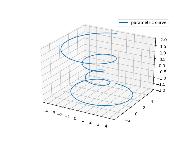
Lines3d
- Scatter plots
Axes3D.scatter(xs, ys, zs=0, zdir='z', s=20, c=None, depthshade=True,
                                              *args, **kwargs)[source]
散布図を作成します。
Argument Description xs, ys データポイントの位置。 zs xs と ys と同じ長さの配列か、すべての点を同じ平面に配置する単一の値のいずれかです。 デフォルトは 0 です。 zdir 2D セットをプロットするときに z( 'x'、 'y' または 'z' )として使用する方向。 s point^2 でサイズ。 スカラまたは x と y と同じ長さの配列です。 c color.c は、単一のカラーフォーマット文字列、または長さNのカラー指定のシーケンス、または kwargs (下記参照)で指定された cmap と norm を使用してカラーにマップされる N 個の数字のシーケンスです。 カラーマップされる値の配列と区別がつかないので、c は単一の数値の RGB または RGBA シーケンスであってはならないことに注意してください。 c は、行が RGB または RGBA の 2 次元配列ですが、すべての点で同じ色を指定する単一の行の場合も含めて、RGB または RGBA です。 depthshade 深度の外観を与えるために散布マーカーを陰影付けするかどうか。 デフォルトはTrueです。
キーワード引数は scatter() に渡されます。
Patch3DCollection を返します。
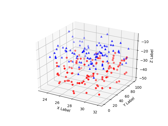
Scatter3d
- Wireframe plots
Axes3D.plot_wireframe(X, Y, Z, *args, **kwargs)[source]
3Dワイヤフレームをプロットする。
注意
rcount と ccount kwargs は両方ともデフォルト値 50 で、各方向で使用されるサンプルの最大数を決定します。 入力データが大きい場合は、これらのポイント数にダウンサンプリング(スライス)します。
Parameters:
- X, Y, Z : 2d arrays
- データ値。
- rcount, ccount : int
- 各方向で使用されるサンプルの最大数。 入力データが大きい場合は、これらのポイント数にダウンサンプリング(スライス)します。 カウントをゼロに設定すると、データが対応する方向にサンプリングされず、ワイヤフレームプロットではなく 3D 線プロットが生成されます。 デフォルトは50です。
バージョン2.0の新機能 - rstride, cstride : int
- 各方向にストライドをダウンサンプリングします。 これらの引数は、rcount および ccount と相互に排他的です。 rstride または cstride のいずれか一方のみが設定されている場合は、もう一方のデフォルトは 1 になります。ストライドをゼロに設定すると、データが対応する方向にサンプリングされず、ワイヤフレームプロットではなく 3D ラインプロットが生成されます。
'classic' モードでは、新しいデフォルトの rcount = ccount = 50 の代わりに、デフォルトの rstride = cstride = 1 が使用されます。 - **kwargs :
- 他の引数はLine3DCollectionに転送されます。
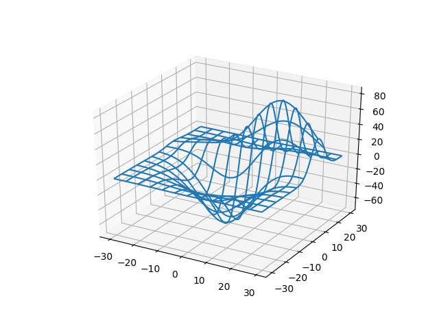
Wire3d
- Surface plots
Axes3D.plot_surface(X, Y, Z, *args, norm=None, vmin=None, vmax=None,
                                   lightsource=None, **kwargs)[source]
サーフェスプロットを作成します。
デフォルトでは、ソリッドカラーの色で色付けされますが、cmap 引数を指定することでカラーマッピングもサポートします。
注意
rcount と ccount kwargs は両方ともデフォルト値 50 で、各方向で使用されるサンプルの最大数を決定します。 入力データが大きい場合は、これらのポイント数にダウンサンプリング(スライス)します。
Parameters:
- X, Y, Z : 2d arrays
- データ値。
- rcount, ccount : int
- 各方向で使用されるサンプルの最大数。 入力データが大きい場合は、これらのポイント数にダウンサンプリング(スライス)します。 デフォルトは 50 です。
バージョン2.0の新機能 - rstride, cstride : int
- 各方向にストライドをダウンサンプリングします。 これらの引数は、rcount および ccoun tと相互に排他的です。 rstride または cstride のいずれか一方のみが設定されている場合、もう一方はデフォルトで 10 になります。
'classic' モードでは、新しいデフォルトの rcount = ccount = 50 ではなく、rstride = cstride = 10 のデフォルト値が使用されます。 - color : color-like
- 表面パッチの色。
- cmap : Colormap
- 表面パッチのカラーマップ。
- facecolors : array-like of colors.
- 個々のパッチの色。
- norm : Normalize
- カラーマップの正規化。
- vmin, vmax : float
- 正規化の境界。
- shade : bool
- 顔の色を濃くするかどうか。
- **kwargs :
- 他の引数はPoly3DCollectionに転送されます。
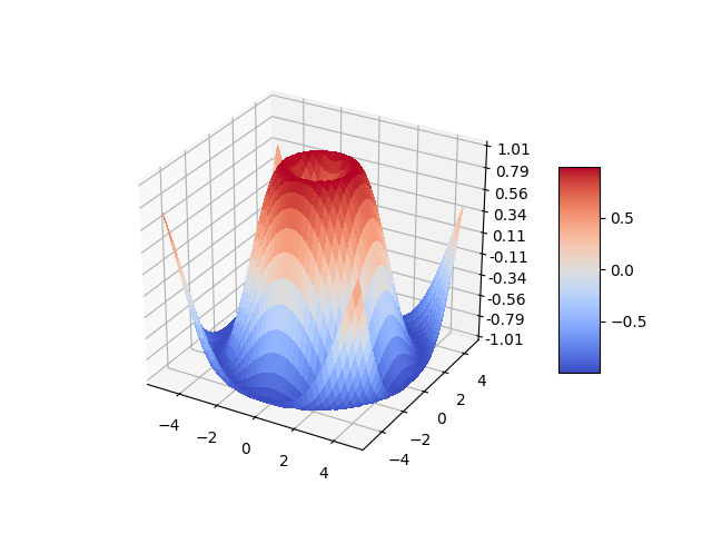
Surface3d
- Tri-Surface plots
Axes3D.plot_trisurf(*args, color=None, norm=None, vmin=None, vmax=None,
                                     lightsource=None, **kwargs)[source]
Argument Description X, Y, Z 1D 配列としてのデータ値 color 表面パッチの色 cmap サーフェスパッチのカラーマップ。 norm 値を色にマップするためのNormalizeのインスタンス vmin マップする最小値 vmax マップする最大値 shade フェーカラーをシェーディングするかどうか
(オプションの)三角測量は、次の2つの方法のいずれかで指定できます。 どちらか:
plot_trisurf(triangulation, ...)
三角測量が Triangulation オブジェクトである場合、または:
plot_trisurf(X, Y, ...)
plot_trisurf(X, Y, triangles, ...)
plot_trisurf(X, Y, triangles=triangles, ...)
この場合、三角形分割オブジェクトが作成されます。 これらの可能性の説明については、 Triangulation を参照してください。
残りの引数は次のとおりです。
plot_trisurf(..., Z)
ここで、Z は輪郭線の値の配列であり、三角形分割の1点につき1つです。
他の引数は Poly3DCollection に渡されます。
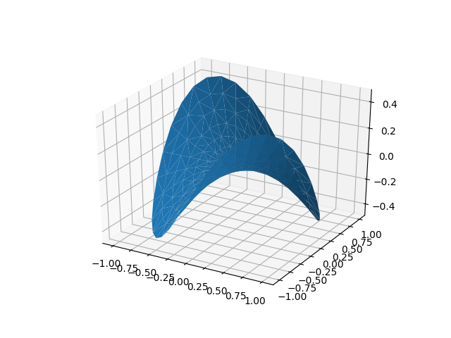
例:1
'''
======================
Triangular 3D surfaces
======================

Plot a 3D surface with a triangular mesh.
'''

# This import registers the 3D projection, but is otherwise unused.
from mpl_toolkits.mplot3d import Axes3D  # noqa: F401 unused import

import matplotlib.pyplot as plt
import numpy as np


n_radii = 8
n_angles = 36

# Make radii and angles spaces (radius r=0 omitted to eliminate duplication).
radii = np.linspace(0.125, 1.0, n_radii)
angles = np.linspace(0, 2*np.pi, n_angles, endpoint=False)[..., np.newaxis]

# Convert polar (radii, angles) coords to cartesian (x, y) coords.
# (0, 0) is manually added at this stage,  so there will be no duplicate
# points in the (x, y) plane.
x = np.append(0, (radii*np.cos(angles)).flatten())
y = np.append(0, (radii*np.sin(angles)).flatten())

# Compute z to make the pringle surface.
z = np.sin(-x*y)

fig = plt.figure()
ax = fig.gca(projection='3d')

ax.plot_trisurf(x, y, z, linewidth=0.2, antialiased=True)

plt.show()
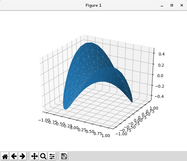
Python 3.11.6 (matplotlib 3.7.1) と Python 3.12.0 (matplotlib 3.8.1) 共に、下記のようなエラーがあり、実行できない。
Traceback (most recent call last): File "E:\______\Surface_plots_01.py", line 33, in
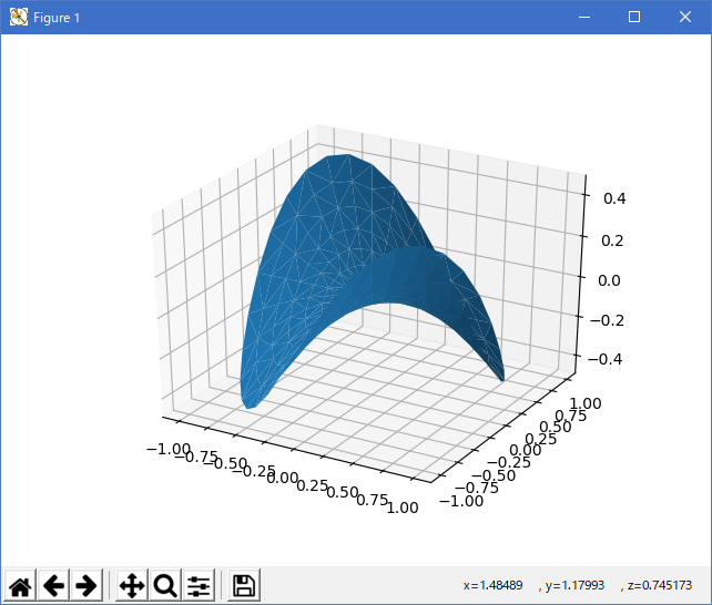
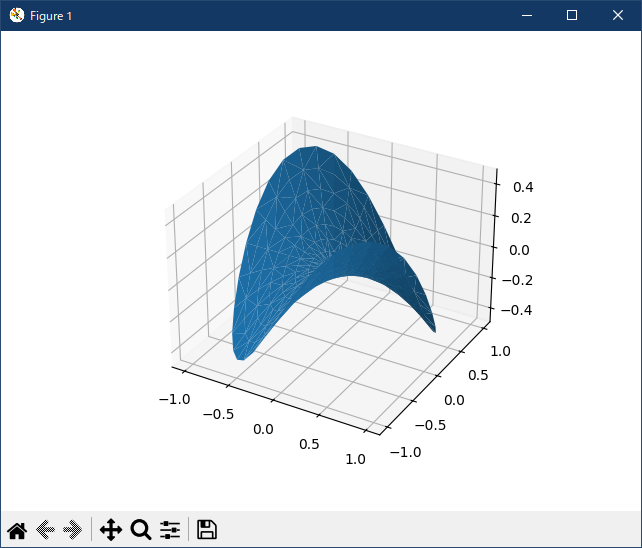
下記のコードであれば、良く似た結果が得られる。ax = fig.gca(projection='3d') ^^^^^^^^^^^^^^^^^^^^^^^^ TypeError: FigureBase.gca() got an unexpected keyword argument 'projection'
import matplotlib.pyplot as plt
import numpy as np

n_radii = 8
n_angles = 36

# Make radii and angles spaces (radius r=0 omitted to eliminate duplication).
radii = np.linspace(0.125, 1.0, n_radii)
angles = np.linspace(0, 2*np.pi, n_angles, endpoint=False)[..., np.newaxis]

# Convert polar (radii, angles) coords to cartesian (x, y) coords.
# (0, 0) is manually added at this stage,  so there will be no duplicate
# points in the (x, y) plane.
x = np.append(0, (radii*np.cos(angles)).flatten())
y = np.append(0, (radii*np.sin(angles)).flatten())

# Compute z to make the pringle surface.
z = np.sin(-x*y)

ax = plt.figure().add_subplot(projection='3d')

ax.plot_trisurf(x, y, z, linewidth=0.2, antialiased=True)

plt.show()
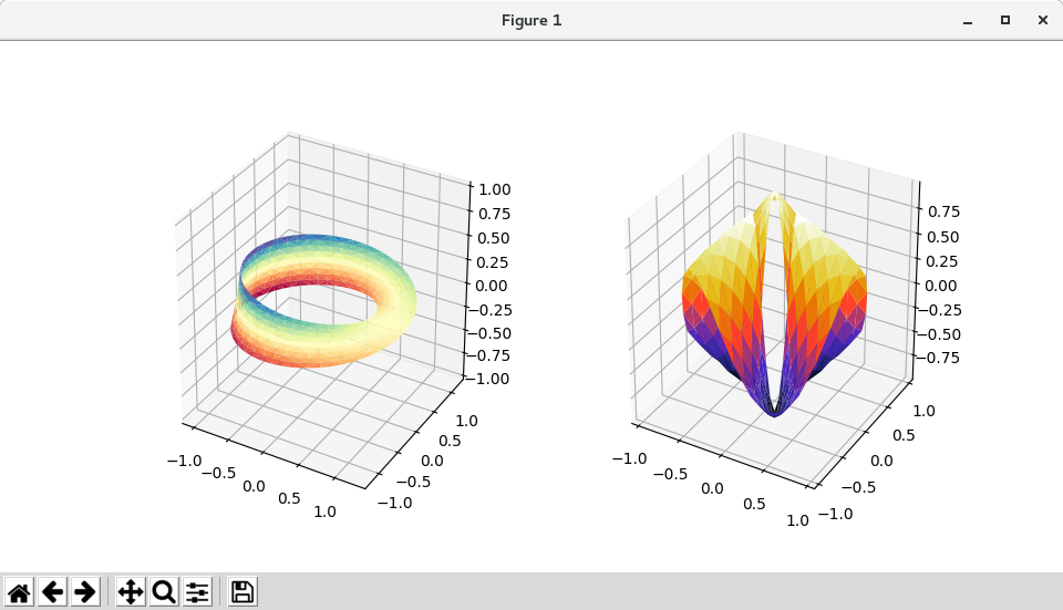
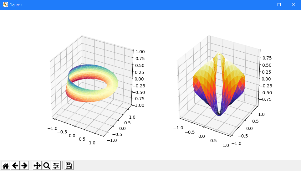
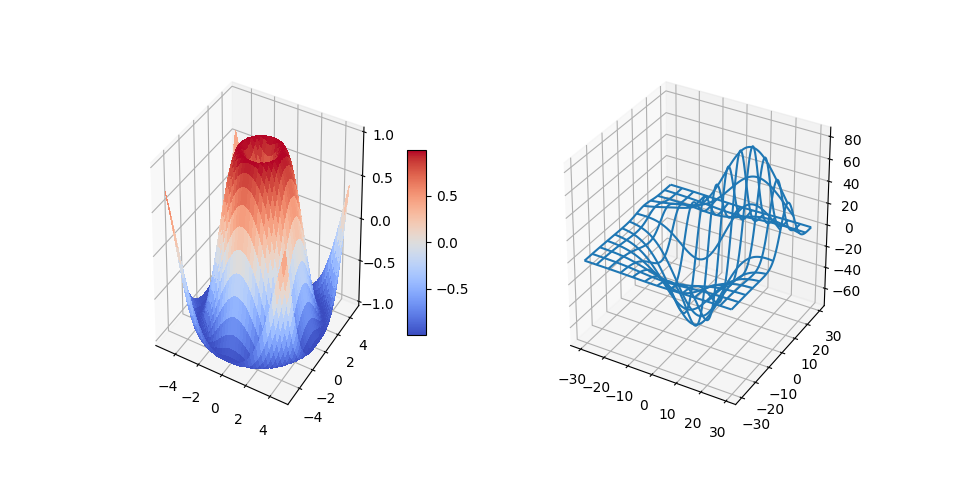
例:2
'''
===========================
More triangular 3D surfaces
===========================

Two additional examples of plotting surfaces with triangular mesh.

The first demonstrates use of plot_trisurf's triangles argument, and the
second sets a Triangulation object's mask and passes the object directly
to plot_trisurf.
'''

import numpy as np
import matplotlib.pyplot as plt
import matplotlib.tri as mtri

# This import registers the 3D projection, but is otherwise unused.
from mpl_toolkits.mplot3d import Axes3D  # noqa: F401 unused import


fig = plt.figure(figsize=plt.figaspect(0.5))

#============
# First plot
#============

# Make a mesh in the space of parameterisation variables u and v
u = np.linspace(0, 2.0 * np.pi, endpoint=True, num=50)
v = np.linspace(-0.5, 0.5, endpoint=True, num=10)
u, v = np.meshgrid(u, v)
u, v = u.flatten(), v.flatten()

# This is the Mobius mapping, taking a u, v pair and returning an x, y, z
# triple
x = (1 + 0.5 * v * np.cos(u / 2.0)) * np.cos(u)
y = (1 + 0.5 * v * np.cos(u / 2.0)) * np.sin(u)
z = 0.5 * v * np.sin(u / 2.0)

# Triangulate parameter space to determine the triangles
tri = mtri.Triangulation(u, v)

# Plot the surface.  The triangles in parameter space determine which x, y, z
# points are connected by an edge.
ax = fig.add_subplot(1, 2, 1, projection='3d')
ax.plot_trisurf(x, y, z, triangles=tri.triangles, cmap=plt.cm.Spectral)
ax.set_zlim(-1, 1)


#============
# Second plot
#============

# Make parameter spaces radii and angles.
n_angles = 36
n_radii = 8
min_radius = 0.25
radii = np.linspace(min_radius, 0.95, n_radii)

angles = np.linspace(0, 2*np.pi, n_angles, endpoint=False)
angles = np.repeat(angles[..., np.newaxis], n_radii, axis=1)
angles[:, 1::2] += np.pi/n_angles

# Map radius, angle pairs to x, y, z points.
x = (radii*np.cos(angles)).flatten()
y = (radii*np.sin(angles)).flatten()
z = (np.cos(radii)*np.cos(3*angles)).flatten()

# Create the Triangulation; no triangles so Delaunay triangulation created.
triang = mtri.Triangulation(x, y)

# Mask off unwanted triangles.
xmid = x[triang.triangles].mean(axis=1)
ymid = y[triang.triangles].mean(axis=1)
mask = np.where(xmid**2 + ymid**2 < min_radius**2, 1, 0)
triang.set_mask(mask)

# Plot the surface.
ax = fig.add_subplot(1, 2, 2, projection='3d')
ax.plot_trisurf(triang, z, cmap=plt.cm.CMRmap)


plt.show()
バージョン 1.2.0 の新機能:このプロット関数が v1.2.0 リリースに追加されました。
Trisurf3d
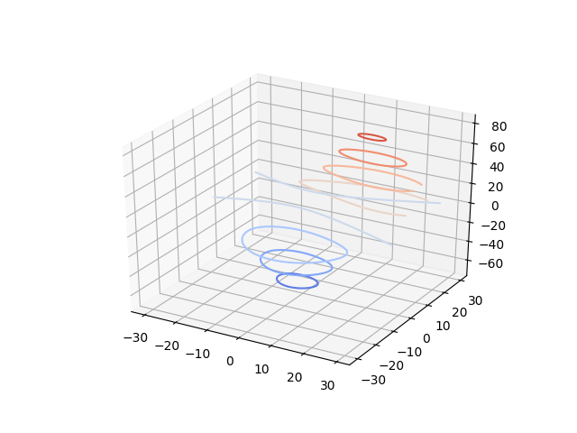
- Contour plots
Axes3D.contour(X, Y, Z, *args, extend3d=False, stride=5, zdir='z',
                                      offset=None, **kwargs)[source]
3D 等高線プロットを作成します。
Argument Description X, Y, Z numpy.arrays としてのデータ値 extend3d 3D で輪郭を拡張するかどうか(デフォルト: False ) stride 輪郭を拡張するためのストライド(ステップサイズ) zdir 使用する方向:x、yまたはz(デフォルト) offset 指定されていれば、zdirに垂直な平面内のこの位置に等高線を投影する
位置およびその他のキーワード引数は、contour()に渡されます。
輪郭を返す
Contour3d
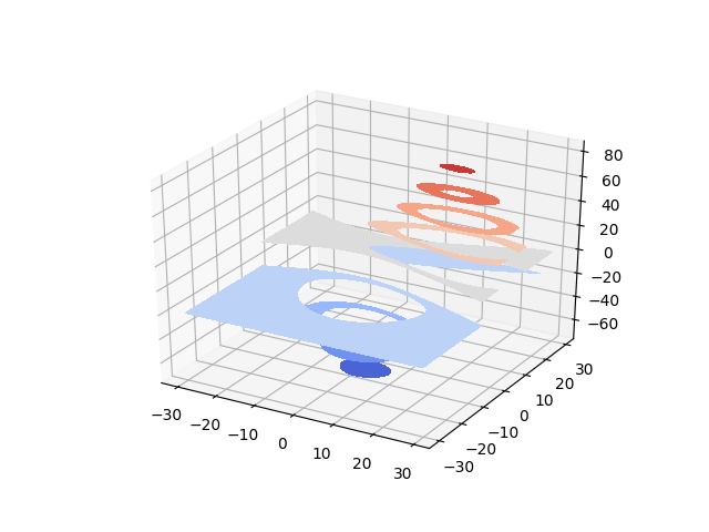
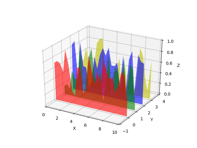
- Filled contour plots
Axes3D.contourf(X, Y, Z, *args, zdir='z', offset=None, **kwargs)[source]
3D contourf プロットを作成します。
Argument Description X, Y, Z numpy.arrays としてのデータ値 zdir 使用する方向:x、yまたはz(デフォルト) offset 指定されている場合は、zdir に垂直な平面内のこの位置に塗りつぶした輪郭を投影します
位置引数とキーワード引数は、contourf()に渡されます。
輪郭線を返す
バージョン 1.1.0 で変更されました: zdirとoffset kwargs が追加されました。
Contourf3d
- Polygon plots
Axes3D.add_collection3d(col, zs=0, zdir='z')
プロットに3Dコレクションオブジェクトを追加します。
2Dコレクションタイプは、オブジェクトを修正し、z座標情報を追加することによって3Dバージョンに変換されます。
サポートされているもの:
- PolyCollection
- LineCollection
- PatchCollection
Polys3d
- Bar plots
Axes3D.bar(left, height, zs=0, zdir='z', *args, **kwargs)[source]
Add 2D bar(s).
Argument Description left 棒の左側のx座標。 height バーの高さ。 zs 棒のZ座標、ある値が指定されている場合は、それらはすべて同じzに置かれます。 zdir 2Dセットをプロットするときにz( 'x'、 'y'または 'z')として使用する方向。
キーワード引数は bar() に渡されます。
Patch3DCollection を返します。
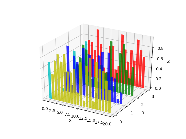
Bars3d
- Quiver
Axes3D.quiver(*args, length=1, arrow_length_ratio=0.3, pivot='tail',
                                   normalize=False, **kwargs)[source]
矢印の3Dフィールドをプロットします。
コールシグネチャ:
quiver(X, Y, Z, U, V, W, **kwargs)
引数:
- X, Y, Z:
- 矢印の位置のx、y、z座標(デフォルトは矢印の末尾です; pivot kwargを参照)
- U, V, W:
- 矢印ベクトルのx、y、z成分
キーワード引数:
- length: [1.0 | float]
- 各震動の長さは、デフォルトでは1.0で、単位は軸と同じです
- arrow_length_ratio: [0.3 | float]
- 矢印の頭と震えとの比。デフォルトは 0.3
- pivot: [ 'tail' | 'middle' | 'tip' ]
- 格子点にある矢印の部分。 矢印はこの点の周りを回転し、したがってピボットという名前がついています。 デフォルトは 'tail' です
- normalize: bool
- True の場合、すべての矢印は同じ長さになります。 このデフォルトは False です。矢印は、u、v、w の値によって異なる長さになります。
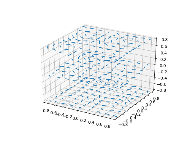
Quiver3d
- 2D plots in 3D
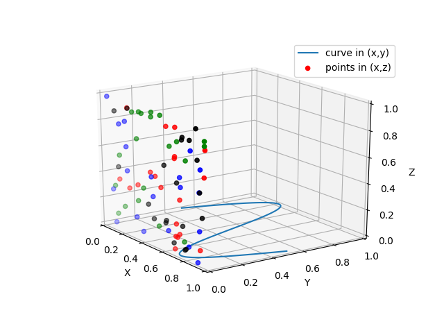
2dcollections3d
- Text
Axes3D.text(x, y, z, s, zdir=None, **kwargs)
プロットにテキストを追加します。 kwargs は Axes.text に渡されますが、zdir キーワードは z 方向として使用される方向を設定します。
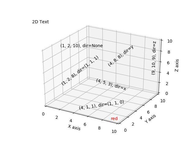
Text3d
- Subplotting
1 つの図形内に複数の 3D プロットを持つことは、2D プロットの場合と同じです。 また、2D と 3D の両方のプロットを同じ図形内に入れることもできます。
バージョン 1.0.0 の新機能: v1.0.0 に 3D プロットのサブプロットが追加されました。 以前のバージョンではこれを行うことはできません。
Subplot3d
- 参照ページ
The mplot3d Toolkit
- リリースノート
- 2023/11/06 Ver=1.04 Python 3.12.0 (matplotlib 3.8.1) で確認
- 2023/11/06 Ver=1.04 Python 3.11.6 (matplotlib 3.7.1) で確認
- 2023/03/11 Ver=1.03 Python 3.11.2 で確認
- 2020/10/28 Ver=1.01 Python 3.7.8 で確認
- 2018/11/08 Ver=1.01 初版リリース
- 関連ページ