|
|
matplotlib statistics_Examples 63_histogram_demo_cumulative. |
H.Kamifuji . |
- histogram_demo_cumulative.py
ヒストグラムを使って累積分布をプロットするデモ
これは、サンプルの経験的累積分布関数(CDF)を視覚化するために、ステップ関数として累積正規化ヒストグラムをプロットする方法を示しています。 また、 "mlab" モジュールを使って理論上の CDF を表示します。
"hist" 関数に対する他のいくつかのオプションが実証されています。 すなわち、ヒストグラムを正規化するために "normed" パラメータを使い、 "cumulative" パラメータにいくつかの異なるオプションを使います。 "normed" パラメータはブール値をとります。 "True" の場合、ビンの高さはヒストグラムの総面積が1になるようにスケーリングされます。 "cumulative" kwarg はもう少し微妙です。 "normed" のように、True または False を渡すことができますが、-1 を渡してその分布を逆にすることもできます。
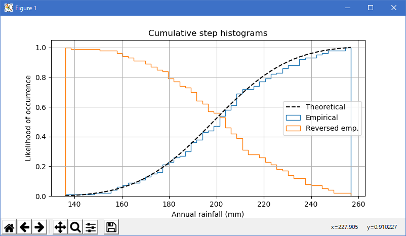
正規化された累積ヒストグラムを表示しているので、これらの曲線は事実上、サンプルの累積分布関数(CDF)です。 エンジニアリングでは、経 験的な CDF は「非超過」曲線と呼ばれることがあります。 言い換えれば、与えられた x 値の y 値を見て、その x 値を超えないサンプルの確率と観測値を得ることができます。 例えば、x 軸上の 225 の値は、y 軸上の約 0.85 に相当するので、サンプル内の観測値が 225 を超えない可能性が 85% です。逆に、「累積」を? この例の最後のシリーズで行われているように、「超過」曲線を作成します。
異なるビンの数とサイズを選択すると、ヒストグラムの形に大きく影響する場合があります。 Astropy のドキュメントには、これらのパラメータの選択方法に関する素晴らしいセクションがあります。http://docs.astropy.org/en/stable/visualization/histogram.html
この事例は、Windows10_1909 で Python 3.9.0 環境では、動作しません。( n, bins, patches = ax.hist(x, n_bins, normed=1, histtype='step', cumulative=True, label='Empirical') がデグレートしたのか? )
"""
==========================================================
Demo of using histograms to plot a cumulative distribution
==========================================================

This shows how to plot a cumulative, normalized histogram as a
step function in order to visualize the empirical cumulative
distribution function (CDF) of a sample. We also use the ``mlab``
module to show the theoretical CDF.

A couple of other options to the ``hist`` function are demonstrated.
Namely, we use the ``normed`` parameter to normalize the histogram and
a couple of different options to the ``cumulative`` parameter.
The ``normed`` parameter takes a boolean value. When ``True``, the bin
heights are scaled such that the total area of the histogram is 1. The
``cumulative`` kwarg is a little more nuanced. Like ``normed``, you
can pass it True or False, but you can also pass it -1 to reverse the
distribution.

Since we're showing a normalized and cumulative histogram, these curves
are effectively the cumulative distribution functions (CDFs) of the
samples. In engineering, empirical CDFs are sometimes called
"non-exceedance" curves. In other words, you can look at the
y-value for a given-x-value to get the probability of and observation
from the sample not exceeding that x-value. For example, the value of
225 on the x-axis corresponds to about 0.85 on the y-axis, so there's an
85% chance that an observation in the sample does not exceed 225.
Conversely, setting, ``cumulative`` to -1 as is done in the
last series for this example, creates a "exceedance" curve.

Selecting different bin counts and sizes can significantly affect the
shape of a histogram. The Astropy docs have a great section on how to
select these parameters:
http://docs.astropy.org/en/stable/visualization/histogram.html

"""

import numpy as np
import matplotlib.pyplot as plt
from matplotlib import mlab

np.random.seed(0)

mu = 200
sigma = 25
n_bins = 50
x = np.random.normal(mu, sigma, size=100)

fig, ax = plt.subplots(figsize=(8, 4))

# plot the cumulative histogram
n, bins, patches = ax.hist(x, n_bins, normed=1, histtype='step',
                           cumulative=True, label='Empirical')

# Add a line showing the expected distribution.
y = mlab.normpdf(bins, mu, sigma).cumsum()
y /= y[-1]

ax.plot(bins, y, 'k--', linewidth=1.5, label='Theoretical')

# Overlay a reversed cumulative histogram.
ax.hist(x, bins=bins, normed=1, histtype='step', cumulative=-1,
        label='Reversed emp.')

# tidy up the figure
ax.grid(True)
ax.legend(loc='right')
ax.set_title('Cumulative step histograms')
ax.set_xlabel('Annual rainfall (mm)')
ax.set_ylabel('Likelihood of occurrence')

plt.show()
- 実行結果( histogram_demo_cumulative.png )
Python 3.11.2 見直しました。上記のコードでは、下記のエラーが発生します。
histogram_demo_cumulative.txt
matplotlib 内部のエラーのようです。matplotlib の改修(先祖帰りバグの改修)を待つしかない。
Python 3.11.6 (matplotlib 3.7.1) では、下記のようなエラーがあり、実行できない。
Traceback (most recent call last): File "M:\______\histogram_demo_cumulative.py", line 52, in
Python 3.12.0 (matplotlib 3.8.1) では、下記のようなエラーがあり、実行できない。n, bins, patches = ax.hist(x, n_bins, normed=1, histtype='step', ^^^^^^^^^^^^^^^^^^^^^^^^^^^^^^^^^^^^^^^^^^^^^ File "C:\Users\______\AppData\Local\Programs\Python\Python311\Lib \site-packages\matplotlib\__init__.py", line 1459, in inner return func(ax, *map(sanitize_sequence, args), **kwargs) ^^^^^^^^^^^^^^^^^^^^^^^^^^^^^^^^^^^^^^^^^^^^^^^^^ File "C:\Users\______\AppData\Local\Programs\Python\Python311\Lib \site-packages\matplotlib\axes\_axes.py", line 6943, in hist p._internal_update(kwargs) File "C:\Users\______\AppData\Local\Programs\Python\Python311\Lib \site-packages\matplotlib\artist.py", line 1223, in _internal_update return self._update_props( ^^^^^^^^^^^^^^^^^^^ File "C:\Users\______\AppData\Local\Programs\Python\Python311\Lib \site-packages\matplotlib\artist.py", line 1197, in _update_props raise AttributeError( AttributeError: Polygon.set() got an unexpected keyword argument 'normed'
Traceback (most recent call last): File "E:\______\histogram_demo_cumulative.py", line 52, in
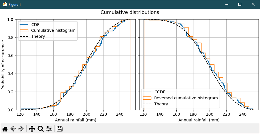
Python 3.11.6 (matplotlib 3.7.1) 及び Python 3.12.0 (matplotlib 3.8.1) で、見直し中、新しいサンプル(statistics-histogram-cumulative-py) を見つけ、下記のコードで、正常に実行できました。n, bins, patches = ax.hist(x, n_bins, normed=1, histtype='step', ^^^^^^^^^^^^^^^^^^^^^^^^^^^^^^^^^^^^^^^^^^^^^ File "C:\Program Files\Python312\Lib\site-packages\matplotlib\__init__.py", line 1478, in inner return func(ax, *map(sanitize_sequence, args), **kwargs) ^^^^^^^^^^^^^^^^^^^^^^^^^^^^^^^^^^^^^^^^^^^^^^^^^ File "C:\Program Files\Python312\Lib\site-packages\matplotlib\axes\_axes.py", line 7012, in hist p._internal_update(kwargs) File "C:\Program Files\Python312\Lib\site-packages\matplotlib\artist.py", line 1219, in _internal_update return self._update_props( ^^^^^^^^^^^^^^^^^^^ File "C:\Program Files\Python312\Lib\site-packages\matplotlib\artist.py", line 1193, in _update_props raise AttributeError( AttributeError: Polygon.set() got an unexpected keyword argument 'normed'
"""
=================================
Plotting cumulative distributions
=================================

This example shows how to plot the empirical cumulative distribution function
(ECDF) of a sample. We also show the theoretical CDF.

In engineering, ECDFs are sometimes called "non-exceedance" curves: the y-value
for a given x-value gives probability that an observation from the sample is
below that x-value. For example, the value of 220 on the x-axis corresponds to
about 0.80 on the y-axis, so there is an 80% chance that an observation in the
sample does not exceed 220. Conversely, the empirical *complementary*
cumulative distribution function (the ECCDF, or "exceedance" curve) shows the
probability y that an observation from the sample is above a value x.

A direct method to plot ECDFs is `.Axes.ecdf`.  Passing ``complementary=True``
results in an ECCDF instead.

Alternatively, one can use ``ax.hist(data, density=True, cumulative=True)`` to
first bin the data, as if plotting a histogram, and then compute and plot the
cumulative sums of the frequencies of entries in each bin.  Here, to plot the
ECCDF, pass ``cumulative=-1``.  Note that this approach results in an
approximation of the E(C)CDF, whereas `.Axes.ecdf` is exact.
"""

import matplotlib.pyplot as plt
import numpy as np

np.random.seed(19680801)

mu = 200
sigma = 25
n_bins = 25
data = np.random.normal(mu, sigma, size=100)

fig = plt.figure(figsize=(9, 4), layout="constrained")
axs = fig.subplots(1, 2, sharex=True, sharey=True)

# Cumulative distributions.
axs[0].ecdf(data, label="CDF")
n, bins, patches = axs[0].hist(data, n_bins, density=True, histtype="step",
                               cumulative=True, label="Cumulative histogram")
x = np.linspace(data.min(), data.max())
y = ((1 / (np.sqrt(2 * np.pi) * sigma)) *
     np.exp(-0.5 * (1 / sigma * (x - mu))**2))
y = y.cumsum()
y /= y[-1]
axs[0].plot(x, y, "k--", linewidth=1.5, label="Theory")

# Complementary cumulative distributions.
axs[1].ecdf(data, complementary=True, label="CCDF")
axs[1].hist(data, bins=bins, density=True, histtype="step", cumulative=-1,
            label="Reversed cumulative histogram")
axs[1].plot(x, 1 - y, "k--", linewidth=1.5, label="Theory")

# Label the figure.
fig.suptitle("Cumulative distributions")
for ax in axs:
    ax.grid(True)
    ax.legend()
    ax.set_xlabel("Annual rainfall (mm)")
    ax.set_ylabel("Probability of occurrence")
    ax.label_outer()

plt.show()

# %%
#
# .. admonition:: References
#
#    The use of the following functions, methods, classes and modules is shown
#    in this example:
#
#    - `matplotlib.axes.Axes.hist` / `matplotlib.pyplot.hist`
#    - `matplotlib.axes.Axes.ecdf` / `matplotlib.pyplot.ecdf`
Python 3.11.6 (matplotlib 3.7.1) では、下記のようなエラーがあり、実行できない。
Traceback (most recent call last): File "M:\______\histogram_cumulative_2.py", line 41, in
Python 3.12.0 (matplotlib 3.8.1) では、正常実行です。axs[0].ecdf(data, label="CDF") ^^^^^^^^^^^ AttributeError: 'Axes' object has no attribute 'ecdf'
- 参照ページ
statistics_Examples code: histogram_demo_cumulative.py
statistics-histogram-cumulative-py
- リリースノート
- 2023/12/10 Ver=1.04 Python 3.12.0 (matplotlib 3.8.1)で確認
- 2023/12/10 Ver=1.04 Python 3.11.6 (matplotlib 3.7.1)で確認
- 2023/04/05 Ver=1.03 Python 3.11.2 で確認
- 2020/11/02 Ver=1.01 Python 3.7.8 で確認
- 2018/12/06 Ver=1.01 初版リリース
- 関連ページ