|
|
pylab_examples_Examples 10_leftventricle_bulleye. |
H.Kamifuji . |
- leftventricle_bulleye.py
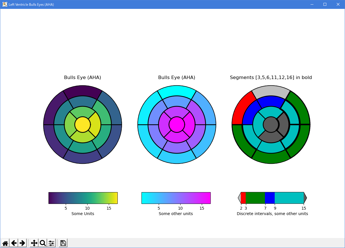
この例では、American Heart Association(AHA)が推奨する左心室の 17 セグメントモデルを作成する方法を示します。
"""
This example demonstrates how to create the 17 segment model for the left
ventricle recommended by the American Heart Association (AHA).
"""

import numpy as np
import matplotlib as mpl
import matplotlib.pyplot as plt


def bullseye_plot(ax, data, segBold=None, cmap=None, norm=None):
    """
    Bullseye representation for the left ventricle.

    Parameters
    ----------
    ax : axes
    data : list of int and float
        The intensity values for each of the 17 segments
    segBold: list of int, optional
        A list with the segments to highlight
    cmap : ColorMap or None, optional
        Optional argument to set the desired colormap
    norm : Normalize or None, optional
        Optional argument to normalize data into the [0.0, 1.0] range


    Notes
    -----
    This function create the 17 segment model for the left ventricle according
    to the American Heart Association (AHA) [1]_

    References
    ----------
    .. [1] M. D. Cerqueira, N. J. Weissman, V. Dilsizian, A. K. Jacobs,
        S. Kaul, W. K. Laskey, D. J. Pennell, J. A. Rumberger, T. Ryan,
        and M. S. Verani, "Standardized myocardial segmentation and
        nomenclature for tomographic imaging of the heart",
        Circulation, vol. 105, no. 4, pp. 539-542, 2002.
    """
    if segBold is None:
        segBold = []

    linewidth = 2
    data = np.array(data).ravel()

    if cmap is None:
        cmap = plt.cm.viridis

    if norm is None:
        norm = mpl.colors.Normalize(vmin=data.min(), vmax=data.max())

    theta = np.linspace(0, 2*np.pi, 768)
    r = np.linspace(0.2, 1, 4)

    # Create the bound for the segment 17
    for i in range(r.shape[0]):
        ax.plot(theta, np.repeat(r[i], theta.shape), '-k', lw=linewidth)

    # Create the bounds for the segments  1-12
    for i in range(6):
        theta_i = i*60*np.pi/180
        ax.plot([theta_i, theta_i], [r[1], 1], '-k', lw=linewidth)

    # Create the bounds for the segments 13-16
    for i in range(4):
        theta_i = i*90*np.pi/180 - 45*np.pi/180
        ax.plot([theta_i, theta_i], [r[0], r[1]], '-k', lw=linewidth)

    # Fill the segments 1-6
    r0 = r[2:4]
    r0 = np.repeat(r0[:, np.newaxis], 128, axis=1).T
    for i in range(6):
        # First segment start at 60 degrees
        theta0 = theta[i*128:i*128+128] + 60*np.pi/180
        theta0 = np.repeat(theta0[:, np.newaxis], 2, axis=1)
        z = np.ones((128, 2))*data[i]
        ax.pcolormesh(theta0, r0, z, cmap=cmap, norm=norm)
        if i+1 in segBold:
            ax.plot(theta0, r0, '-k', lw=linewidth+2)
            ax.plot(theta0[0], [r[2], r[3]], '-k', lw=linewidth+1)
            ax.plot(theta0[-1], [r[2], r[3]], '-k', lw=linewidth+1)

    # Fill the segments 7-12
    r0 = r[1:3]
    r0 = np.repeat(r0[:, np.newaxis], 128, axis=1).T
    for i in range(6):
        # First segment start at 60 degrees
        theta0 = theta[i*128:i*128+128] + 60*np.pi/180
        theta0 = np.repeat(theta0[:, np.newaxis], 2, axis=1)
        z = np.ones((128, 2))*data[i+6]
        ax.pcolormesh(theta0, r0, z, cmap=cmap, norm=norm)
        if i+7 in segBold:
            ax.plot(theta0, r0, '-k', lw=linewidth+2)
            ax.plot(theta0[0], [r[1], r[2]], '-k', lw=linewidth+1)
            ax.plot(theta0[-1], [r[1], r[2]], '-k', lw=linewidth+1)

    # Fill the segments 13-16
    r0 = r[0:2]
    r0 = np.repeat(r0[:, np.newaxis], 192, axis=1).T
    for i in range(4):
        # First segment start at 45 degrees
        theta0 = theta[i*192:i*192+192] + 45*np.pi/180
        theta0 = np.repeat(theta0[:, np.newaxis], 2, axis=1)
        z = np.ones((192, 2))*data[i+12]
        ax.pcolormesh(theta0, r0, z, cmap=cmap, norm=norm)
        if i+13 in segBold:
            ax.plot(theta0, r0, '-k', lw=linewidth+2)
            ax.plot(theta0[0], [r[0], r[1]], '-k', lw=linewidth+1)
            ax.plot(theta0[-1], [r[0], r[1]], '-k', lw=linewidth+1)

    # Fill the segments 17
    if data.size == 17:
        r0 = np.array([0, r[0]])
        r0 = np.repeat(r0[:, np.newaxis], theta.size, axis=1).T
        theta0 = np.repeat(theta[:, np.newaxis], 2, axis=1)
        z = np.ones((theta.size, 2))*data[16]
        ax.pcolormesh(theta0, r0, z, cmap=cmap, norm=norm)
        if 17 in segBold:
            ax.plot(theta0, r0, '-k', lw=linewidth+2)

    ax.set_ylim([0, 1])
    ax.set_yticklabels([])
    ax.set_xticklabels([])


# Create the fake data
data = np.array(range(17)) + 1


# Make a figure and axes with dimensions as desired.
fig, ax = plt.subplots(figsize=(12, 8), nrows=1, ncols=3,
                       subplot_kw=dict(projection='polar'))
fig.canvas.set_window_title('Left Ventricle Bulls Eyes (AHA)')

# Create the axis for the colorbars
axl = fig.add_axes([0.14, 0.15, 0.2, 0.05])
axl2 = fig.add_axes([0.41, 0.15, 0.2, 0.05])
axl3 = fig.add_axes([0.69, 0.15, 0.2, 0.05])


# Set the colormap and norm to correspond to the data for which
# the colorbar will be used.
cmap = mpl.cm.viridis
norm = mpl.colors.Normalize(vmin=1, vmax=17)

# ColorbarBase derives from ScalarMappable and puts a colorbar
# in a specified axes, so it has everything needed for a
# standalone colorbar.  There are many more kwargs, but the
# following gives a basic continuous colorbar with ticks
# and labels.
cb1 = mpl.colorbar.ColorbarBase(axl, cmap=cmap, norm=norm,
                                orientation='horizontal')
cb1.set_label('Some Units')


# Set the colormap and norm to correspond to the data for which
# the colorbar will be used.
cmap2 = mpl.cm.cool
norm2 = mpl.colors.Normalize(vmin=1, vmax=17)

# ColorbarBase derives from ScalarMappable and puts a colorbar
# in a specified axes, so it has everything needed for a
# standalone colorbar.  There are many more kwargs, but the
# following gives a basic continuous colorbar with ticks
# and labels.
cb2 = mpl.colorbar.ColorbarBase(axl2, cmap=cmap2, norm=norm2,
                                orientation='horizontal')
cb2.set_label('Some other units')


# The second example illustrates the use of a ListedColormap, a
# BoundaryNorm, and extended ends to show the "over" and "under"
# value colors.
cmap3 = mpl.colors.ListedColormap(['r', 'g', 'b', 'c'])
cmap3.set_over('0.35')
cmap3.set_under('0.75')

# If a ListedColormap is used, the length of the bounds array must be
# one greater than the length of the color list.  The bounds must be
# monotonically increasing.
bounds = [2, 3, 7, 9, 15]
norm3 = mpl.colors.BoundaryNorm(bounds, cmap3.N)
cb3 = mpl.colorbar.ColorbarBase(axl3, cmap=cmap3, norm=norm3,
                                # to use 'extend', you must
                                # specify two extra boundaries:
                                boundaries=[0]+bounds+[18],
                                extend='both',
                                ticks=bounds,  # optional
                                spacing='proportional',
                                orientation='horizontal')
cb3.set_label('Discrete intervals, some other units')


# Create the 17 segment model
bullseye_plot(ax[0], data, cmap=cmap, norm=norm)
ax[0].set_title('Bulls Eye (AHA)')

bullseye_plot(ax[1], data, cmap=cmap2, norm=norm2)
ax[1].set_title('Bulls Eye (AHA)')

bullseye_plot(ax[2], data, segBold=[3, 5, 6, 11, 12, 16],
              cmap=cmap3, norm=norm3)
ax[2].set_title('Segments [3,5,6,11,12,16] in bold')

plt.show()
- 実行結果( leftventricle_bulleye.png )
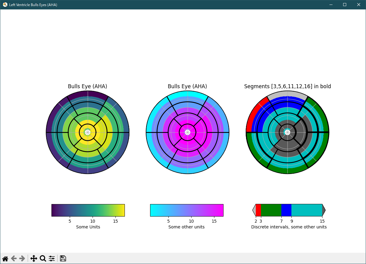
Python 3.11.2 見直しました。上記のコードでは、下記のエラーが発生します。
Traceback (most recent call last):
File "_:\leftventricle_bulleye.py", line 134, in <module>
fig.canvas.set_window_title('Left Ventricle Bulls Eyes (AHA)')
^^^^^^^^^^^^^^^^^^^^^^^^^^^
AttributeError: 'FigureCanvasTkAgg' object has no attribute 'set_window_title'
matplotlib 内部のエラーのようです。matplotlib の改修(先祖帰りバグの改修)を待つしかない。
Python 3.11.6 (matplotlib 3.7.1) では、下記のようなエラーがあり、実行できない。
Traceback (most recent call last): File "M:\______\leftventricle_bulleye.py", line 134, in
Python 3.11.6 (matplotlib 3.7.1) では、下記のようなエラーがあり、実行できない。fig.canvas.set_window_title('Left Ventricle Bulls Eyes (AHA)') ^^^^^^^^^^^^^^^^^^^^^^^^^^^ AttributeError: 'FigureCanvasTkAgg' object has no attribute 'set_window_title'
Traceback (most recent call last): File "E:\______\leftventricle_bulleye.py", line 134, in
前の事例(27_boxplot_demo2) と同様に、num キーワード指定で、改修しました。fig.canvas.set_window_title('Left Ventricle Bulls Eyes (AHA)') ^^^^^^^^^^^^^^^^^^^^^^^^^^^ AttributeError: 'FigureCanvasTkAgg' object has no attribute 'set_window_title'
"""
This example demonstrates how to create the 17 segment model for the left
ventricle recommended by the American Heart Association (AHA).
"""

import numpy as np
import matplotlib as mpl
import matplotlib.pyplot as plt


def bullseye_plot(ax, data, segBold=None, cmap=None, norm=None):
    """
    Bullseye representation for the left ventricle.

    Parameters
    ----------
    ax : axes
    data : list of int and float
        The intensity values for each of the 17 segments
    segBold: list of int, optional
        A list with the segments to highlight
    cmap : ColorMap or None, optional
        Optional argument to set the desired colormap
    norm : Normalize or None, optional
        Optional argument to normalize data into the [0.0, 1.0] range


    Notes
    -----
    This function create the 17 segment model for the left ventricle according
    to the American Heart Association (AHA) [1]_

    References
    ----------
    .. [1] M. D. Cerqueira, N. J. Weissman, V. Dilsizian, A. K. Jacobs,
        S. Kaul, W. K. Laskey, D. J. Pennell, J. A. Rumberger, T. Ryan,
        and M. S. Verani, "Standardized myocardial segmentation and
        nomenclature for tomographic imaging of the heart",
        Circulation, vol. 105, no. 4, pp. 539-542, 2002.
    """
    if segBold is None:
        segBold = []

    linewidth = 2
    data = np.array(data).ravel()

    if cmap is None:
        cmap = plt.cm.viridis

    if norm is None:
        norm = mpl.colors.Normalize(vmin=data.min(), vmax=data.max())

    theta = np.linspace(0, 2*np.pi, 768)
    r = np.linspace(0.2, 1, 4)

    # Create the bound for the segment 17
    for i in range(r.shape[0]):
        ax.plot(theta, np.repeat(r[i], theta.shape), '-k', lw=linewidth)

    # Create the bounds for the segments  1-12
    for i in range(6):
        theta_i = i*60*np.pi/180
        ax.plot([theta_i, theta_i], [r[1], 1], '-k', lw=linewidth)

    # Create the bounds for the segments 13-16
    for i in range(4):
        theta_i = i*90*np.pi/180 - 45*np.pi/180
        ax.plot([theta_i, theta_i], [r[0], r[1]], '-k', lw=linewidth)

    # Fill the segments 1-6
    r0 = r[2:4]
    r0 = np.repeat(r0[:, np.newaxis], 128, axis=1).T
    for i in range(6):
        # First segment start at 60 degrees
        theta0 = theta[i*128:i*128+128] + 60*np.pi/180
        theta0 = np.repeat(theta0[:, np.newaxis], 2, axis=1)
        z = np.ones((128, 2))*data[i]
        ax.pcolormesh(theta0, r0, z, cmap=cmap, norm=norm)
        if i+1 in segBold:
            ax.plot(theta0, r0, '-k', lw=linewidth+2)
            ax.plot(theta0[0], [r[2], r[3]], '-k', lw=linewidth+1)
            ax.plot(theta0[-1], [r[2], r[3]], '-k', lw=linewidth+1)

    # Fill the segments 7-12
    r0 = r[1:3]
    r0 = np.repeat(r0[:, np.newaxis], 128, axis=1).T
    for i in range(6):
        # First segment start at 60 degrees
        theta0 = theta[i*128:i*128+128] + 60*np.pi/180
        theta0 = np.repeat(theta0[:, np.newaxis], 2, axis=1)
        z = np.ones((128, 2))*data[i+6]
        ax.pcolormesh(theta0, r0, z, cmap=cmap, norm=norm)
        if i+7 in segBold:
            ax.plot(theta0, r0, '-k', lw=linewidth+2)
            ax.plot(theta0[0], [r[1], r[2]], '-k', lw=linewidth+1)
            ax.plot(theta0[-1], [r[1], r[2]], '-k', lw=linewidth+1)

    # Fill the segments 13-16
    r0 = r[0:2]
    r0 = np.repeat(r0[:, np.newaxis], 192, axis=1).T
    for i in range(4):
        # First segment start at 45 degrees
        theta0 = theta[i*192:i*192+192] + 45*np.pi/180
        theta0 = np.repeat(theta0[:, np.newaxis], 2, axis=1)
        z = np.ones((192, 2))*data[i+12]
        ax.pcolormesh(theta0, r0, z, cmap=cmap, norm=norm)
        if i+13 in segBold:
            ax.plot(theta0, r0, '-k', lw=linewidth+2)
            ax.plot(theta0[0], [r[0], r[1]], '-k', lw=linewidth+1)
            ax.plot(theta0[-1], [r[0], r[1]], '-k', lw=linewidth+1)

    # Fill the segments 17
    if data.size == 17:
        r0 = np.array([0, r[0]])
        r0 = np.repeat(r0[:, np.newaxis], theta.size, axis=1).T
        theta0 = np.repeat(theta[:, np.newaxis], 2, axis=1)
        z = np.ones((theta.size, 2))*data[16]
        ax.pcolormesh(theta0, r0, z, cmap=cmap, norm=norm)
        if 17 in segBold:
            ax.plot(theta0, r0, '-k', lw=linewidth+2)

    ax.set_ylim([0, 1])
    ax.set_yticklabels([])
    ax.set_xticklabels([])


# Create the fake data
data = np.array(range(17)) + 1


# Make a figure and axes with dimensions as desired.
fig, ax = plt.subplots(figsize=(12, 8), nrows=1, ncols=3,
                       subplot_kw=dict(projection='polar'),
                    num='Left Ventricle Bulls Eyes (AHA)')
# fig.canvas.set_window_title('Left Ventricle Bulls Eyes (AHA)')

# Create the axis for the colorbars
axl = fig.add_axes([0.14, 0.15, 0.2, 0.05])
axl2 = fig.add_axes([0.41, 0.15, 0.2, 0.05])
axl3 = fig.add_axes([0.69, 0.15, 0.2, 0.05])


# Set the colormap and norm to correspond to the data for which
# the colorbar will be used.
cmap = mpl.cm.viridis
norm = mpl.colors.Normalize(vmin=1, vmax=17)

# ColorbarBase derives from ScalarMappable and puts a colorbar
# in a specified axes, so it has everything needed for a
# standalone colorbar.  There are many more kwargs, but the
# following gives a basic continuous colorbar with ticks
# and labels.
cb1 = mpl.colorbar.ColorbarBase(axl, cmap=cmap, norm=norm,
                                orientation='horizontal')
cb1.set_label('Some Units')


# Set the colormap and norm to correspond to the data for which
# the colorbar will be used.
cmap2 = mpl.cm.cool
norm2 = mpl.colors.Normalize(vmin=1, vmax=17)

# ColorbarBase derives from ScalarMappable and puts a colorbar
# in a specified axes, so it has everything needed for a
# standalone colorbar.  There are many more kwargs, but the
# following gives a basic continuous colorbar with ticks
# and labels.
cb2 = mpl.colorbar.ColorbarBase(axl2, cmap=cmap2, norm=norm2,
                                orientation='horizontal')
cb2.set_label('Some other units')


# The second example illustrates the use of a ListedColormap, a
# BoundaryNorm, and extended ends to show the "over" and "under"
# value colors.
cmap3 = mpl.colors.ListedColormap(['r', 'g', 'b', 'c'])
cmap3.set_over('0.35')
cmap3.set_under('0.75')

# If a ListedColormap is used, the length of the bounds array must be
# one greater than the length of the color list.  The bounds must be
# monotonically increasing.
bounds = [2, 3, 7, 9, 15]
norm3 = mpl.colors.BoundaryNorm(bounds, cmap3.N)
cb3 = mpl.colorbar.ColorbarBase(axl3, cmap=cmap3, norm=norm3,
                                # to use 'extend', you must
                                # specify two extra boundaries:
                                boundaries=[0]+bounds+[18],
                                extend='both',
                                ticks=bounds,  # optional
                                spacing='proportional',
                                orientation='horizontal')
cb3.set_label('Discrete intervals, some other units')


# Create the 17 segment model
bullseye_plot(ax[0], data, cmap=cmap, norm=norm)
ax[0].set_title('Bulls Eye (AHA)')

bullseye_plot(ax[1], data, cmap=cmap2, norm=norm2)
ax[1].set_title('Bulls Eye (AHA)')

bullseye_plot(ax[2], data, segBold=[3, 5, 6, 11, 12, 16],
              cmap=cmap3, norm=norm3)
ax[2].set_title('Segments [3,5,6,11,12,16] in bold')

plt.show()
Python 3.11.6 (matplotlib 3.7.1) 及び Python 3.12.0 (matplotlib 3.8.1) 共に、正常実行です。
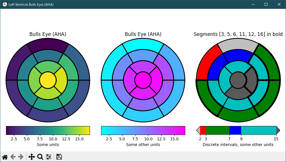
Python 3.11.6 (matplotlib 3.7.1) 及び Python 3.12.0 (matplotlib 3.8.1) で、見直し中、新しいサンプル(specialty-plots-leftventricle-bullseye-py) を見つけ、下記のコードで、正常に実行できました。
"""
=======================
Left ventricle bullseye
=======================

This example demonstrates how to create the 17 segment model for the left
ventricle recommended by the American Heart Association (AHA).

.. redirect-from:: /gallery/specialty_plots/leftventricle_bulleye

See also the :doc:`/gallery/pie_and_polar_charts/nested_pie` example.
"""

import matplotlib.pyplot as plt
import numpy as np

import matplotlib as mpl


def bullseye_plot(ax, data, seg_bold=None, cmap="viridis", norm=None):
    """
    Bullseye representation for the left ventricle.

    Parameters
    ----------
    ax : axes
    data : list[float]
        The intensity values for each of the 17 segments.
    seg_bold : list[int], optional
        A list with the segments to highlight.
    cmap : colormap, default: "viridis"
        Colormap for the data.
    norm : Normalize or None, optional
        Normalizer for the data.

    Notes
    -----
    This function creates the 17 segment model for the left ventricle according
    to the American Heart Association (AHA) [1]_

    References
    ----------
    .. [1] M. D. Cerqueira, N. J. Weissman, V. Dilsizian, A. K. Jacobs,
        S. Kaul, W. K. Laskey, D. J. Pennell, J. A. Rumberger, T. Ryan,
        and M. S. Verani, "Standardized myocardial segmentation and
        nomenclature for tomographic imaging of the heart",
        Circulation, vol. 105, no. 4, pp. 539-542, 2002.
    """

    data = np.ravel(data)
    if seg_bold is None:
        seg_bold = []
    if norm is None:
        norm = mpl.colors.Normalize(vmin=data.min(), vmax=data.max())

    r = np.linspace(0.2, 1, 4)

    ax.set(ylim=[0, 1], xticklabels=[], yticklabels=[])
    ax.grid(False)  # Remove grid

    # Fill segments 1-6, 7-12, 13-16.
    for start, stop, r_in, r_out in [
            (0, 6, r[2], r[3]),
            (6, 12, r[1], r[2]),
            (12, 16, r[0], r[1]),
            (16, 17, 0, r[0]),
    ]:
        n = stop - start
        dtheta = 2*np.pi / n
        ax.bar(np.arange(n) * dtheta + np.pi/2, r_out - r_in, dtheta, r_in,
               color=cmap(norm(data[start:stop])))

    # Now, draw the segment borders.  In order for the outer bold borders not
    # to be covered by inner segments, the borders are all drawn separately
    # after the segments have all been filled.  We also disable clipping, which
    # would otherwise affect the outermost segment edges.
    # Draw edges of segments 1-6, 7-12, 13-16.
    for start, stop, r_in, r_out in [
            (0, 6, r[2], r[3]),
            (6, 12, r[1], r[2]),
            (12, 16, r[0], r[1]),
    ]:
        n = stop - start
        dtheta = 2*np.pi / n
        ax.bar(np.arange(n) * dtheta + np.pi/2, r_out - r_in, dtheta, r_in,
               clip_on=False, color="none", edgecolor="k", linewidth=[
                   4 if i + 1 in seg_bold else 2 for i in range(start, stop)])
    # Draw edge of segment 17 -- here; the edge needs to be drawn differently,
    # using plot().
    ax.plot(np.linspace(0, 2*np.pi), np.linspace(r[0], r[0]), "k",
            linewidth=(4 if 17 in seg_bold else 2))


# Create the fake data
data = np.arange(17) + 1


# Make a figure and axes with dimensions as desired.
fig = plt.figure(figsize=(10, 5), layout="constrained")
fig.get_layout_engine().set(wspace=.1, w_pad=.2)
axs = fig.subplots(1, 3, subplot_kw=dict(projection='polar'))
fig.canvas.manager.set_window_title('Left Ventricle Bulls Eyes (AHA)')


# Set the colormap and norm to correspond to the data for which
# the colorbar will be used.
cmap = mpl.cm.viridis
norm = mpl.colors.Normalize(vmin=1, vmax=17)
# Create an empty ScalarMappable to set the colorbar's colormap and norm.
# The following gives a basic continuous colorbar with ticks and labels.
fig.colorbar(mpl.cm.ScalarMappable(cmap=cmap, norm=norm),
             cax=axs[0].inset_axes([0, -.15, 1, .1]),
             orientation='horizontal', label='Some units')


# And again for the second colorbar.
cmap2 = mpl.cm.cool
norm2 = mpl.colors.Normalize(vmin=1, vmax=17)
fig.colorbar(mpl.cm.ScalarMappable(cmap=cmap2, norm=norm2),
             cax=axs[1].inset_axes([0, -.15, 1, .1]),
             orientation='horizontal', label='Some other units')


# The second example illustrates the use of a ListedColormap, a
# BoundaryNorm, and extended ends to show the "over" and "under"
# value colors.
cmap3 = (mpl.colors.ListedColormap(['r', 'g', 'b', 'c'])
         .with_extremes(over='0.35', under='0.75'))
# If a ListedColormap is used, the length of the bounds array must be
# one greater than the length of the color list.  The bounds must be
# monotonically increasing.
bounds = [2, 3, 7, 9, 15]
norm3 = mpl.colors.BoundaryNorm(bounds, cmap3.N)
fig.colorbar(mpl.cm.ScalarMappable(cmap=cmap3, norm=norm3),
             cax=axs[2].inset_axes([0, -.15, 1, .1]),
             extend='both',
             ticks=bounds,  # optional
             spacing='proportional',
             orientation='horizontal',
             label='Discrete intervals, some other units')


# Create the 17 segment model
bullseye_plot(axs[0], data, cmap=cmap, norm=norm)
axs[0].set_title('Bulls Eye (AHA)')

bullseye_plot(axs[1], data, cmap=cmap2, norm=norm2)
axs[1].set_title('Bulls Eye (AHA)')

bullseye_plot(axs[2], data, seg_bold=[3, 5, 6, 11, 12, 16],
              cmap=cmap3, norm=norm3)
axs[2].set_title('Segments [3, 5, 6, 11, 12, 16] in bold')

plt.show()
fig.canvas.set_window_title が fig.canvas.manager.set_window_title に、改修さえているようです。
Python 3.11.6 (matplotlib 3.7.1) 及び Python 3.12.0 (matplotlib 3.8.1) 共に、正常実行です。
初版に対し、fig.canvas.set_window_title を fig.canvas.manager.set_window_title に、改修しました。
"""
This example demonstrates how to create the 17 segment model for the left
ventricle recommended by the American Heart Association (AHA).
"""

import numpy as np
import matplotlib as mpl
import matplotlib.pyplot as plt


def bullseye_plot(ax, data, segBold=None, cmap=None, norm=None):
    """
    Bullseye representation for the left ventricle.

    Parameters
    ----------
    ax : axes
    data : list of int and float
        The intensity values for each of the 17 segments
    segBold: list of int, optional
        A list with the segments to highlight
    cmap : ColorMap or None, optional
        Optional argument to set the desired colormap
    norm : Normalize or None, optional
        Optional argument to normalize data into the [0.0, 1.0] range


    Notes
    -----
    This function create the 17 segment model for the left ventricle according
    to the American Heart Association (AHA) [1]_

    References
    ----------
    .. [1] M. D. Cerqueira, N. J. Weissman, V. Dilsizian, A. K. Jacobs,
        S. Kaul, W. K. Laskey, D. J. Pennell, J. A. Rumberger, T. Ryan,
        and M. S. Verani, "Standardized myocardial segmentation and
        nomenclature for tomographic imaging of the heart",
        Circulation, vol. 105, no. 4, pp. 539-542, 2002.
    """
    if segBold is None:
        segBold = []

    linewidth = 2
    data = np.array(data).ravel()

    if cmap is None:
        cmap = plt.cm.viridis

    if norm is None:
        norm = mpl.colors.Normalize(vmin=data.min(), vmax=data.max())

    theta = np.linspace(0, 2*np.pi, 768)
    r = np.linspace(0.2, 1, 4)

    # Create the bound for the segment 17
    for i in range(r.shape[0]):
        ax.plot(theta, np.repeat(r[i], theta.shape), '-k', lw=linewidth)

    # Create the bounds for the segments  1-12
    for i in range(6):
        theta_i = i*60*np.pi/180
        ax.plot([theta_i, theta_i], [r[1], 1], '-k', lw=linewidth)

    # Create the bounds for the segments 13-16
    for i in range(4):
        theta_i = i*90*np.pi/180 - 45*np.pi/180
        ax.plot([theta_i, theta_i], [r[0], r[1]], '-k', lw=linewidth)

    # Fill the segments 1-6
    r0 = r[2:4]
    r0 = np.repeat(r0[:, np.newaxis], 128, axis=1).T
    for i in range(6):
        # First segment start at 60 degrees
        theta0 = theta[i*128:i*128+128] + 60*np.pi/180
        theta0 = np.repeat(theta0[:, np.newaxis], 2, axis=1)
        z = np.ones((128, 2))*data[i]
        ax.pcolormesh(theta0, r0, z, cmap=cmap, norm=norm)
        if i+1 in segBold:
            ax.plot(theta0, r0, '-k', lw=linewidth+2)
            ax.plot(theta0[0], [r[2], r[3]], '-k', lw=linewidth+1)
            ax.plot(theta0[-1], [r[2], r[3]], '-k', lw=linewidth+1)

    # Fill the segments 7-12
    r0 = r[1:3]
    r0 = np.repeat(r0[:, np.newaxis], 128, axis=1).T
    for i in range(6):
        # First segment start at 60 degrees
        theta0 = theta[i*128:i*128+128] + 60*np.pi/180
        theta0 = np.repeat(theta0[:, np.newaxis], 2, axis=1)
        z = np.ones((128, 2))*data[i+6]
        ax.pcolormesh(theta0, r0, z, cmap=cmap, norm=norm)
        if i+7 in segBold:
            ax.plot(theta0, r0, '-k', lw=linewidth+2)
            ax.plot(theta0[0], [r[1], r[2]], '-k', lw=linewidth+1)
            ax.plot(theta0[-1], [r[1], r[2]], '-k', lw=linewidth+1)

    # Fill the segments 13-16
    r0 = r[0:2]
    r0 = np.repeat(r0[:, np.newaxis], 192, axis=1).T
    for i in range(4):
        # First segment start at 45 degrees
        theta0 = theta[i*192:i*192+192] + 45*np.pi/180
        theta0 = np.repeat(theta0[:, np.newaxis], 2, axis=1)
        z = np.ones((192, 2))*data[i+12]
        ax.pcolormesh(theta0, r0, z, cmap=cmap, norm=norm)
        if i+13 in segBold:
            ax.plot(theta0, r0, '-k', lw=linewidth+2)
            ax.plot(theta0[0], [r[0], r[1]], '-k', lw=linewidth+1)
            ax.plot(theta0[-1], [r[0], r[1]], '-k', lw=linewidth+1)

    # Fill the segments 17
    if data.size == 17:
        r0 = np.array([0, r[0]])
        r0 = np.repeat(r0[:, np.newaxis], theta.size, axis=1).T
        theta0 = np.repeat(theta[:, np.newaxis], 2, axis=1)
        z = np.ones((theta.size, 2))*data[16]
        ax.pcolormesh(theta0, r0, z, cmap=cmap, norm=norm)
        if 17 in segBold:
            ax.plot(theta0, r0, '-k', lw=linewidth+2)

    ax.set_ylim([0, 1])
    ax.set_yticklabels([])
    ax.set_xticklabels([])


# Create the fake data
data = np.array(range(17)) + 1


# Make a figure and axes with dimensions as desired.
fig, ax = plt.subplots(figsize=(12, 8), nrows=1, ncols=3,
                       subplot_kw=dict(projection='polar'))
# fig.canvas.set_window_title('Left Ventricle Bulls Eyes (AHA)')
fig.canvas.manager.set_window_title('Left Ventricle Bulls Eyes (AHA)')

# Create the axis for the colorbars
axl = fig.add_axes([0.14, 0.15, 0.2, 0.05])
axl2 = fig.add_axes([0.41, 0.15, 0.2, 0.05])
axl3 = fig.add_axes([0.69, 0.15, 0.2, 0.05])


# Set the colormap and norm to correspond to the data for which
# the colorbar will be used.
cmap = mpl.cm.viridis
norm = mpl.colors.Normalize(vmin=1, vmax=17)

# ColorbarBase derives from ScalarMappable and puts a colorbar
# in a specified axes, so it has everything needed for a
# standalone colorbar.  There are many more kwargs, but the
# following gives a basic continuous colorbar with ticks
# and labels.
cb1 = mpl.colorbar.ColorbarBase(axl, cmap=cmap, norm=norm,
                                orientation='horizontal')
cb1.set_label('Some Units')


# Set the colormap and norm to correspond to the data for which
# the colorbar will be used.
cmap2 = mpl.cm.cool
norm2 = mpl.colors.Normalize(vmin=1, vmax=17)

# ColorbarBase derives from ScalarMappable and puts a colorbar
# in a specified axes, so it has everything needed for a
# standalone colorbar.  There are many more kwargs, but the
# following gives a basic continuous colorbar with ticks
# and labels.
cb2 = mpl.colorbar.ColorbarBase(axl2, cmap=cmap2, norm=norm2,
                                orientation='horizontal')
cb2.set_label('Some other units')


# The second example illustrates the use of a ListedColormap, a
# BoundaryNorm, and extended ends to show the "over" and "under"
# value colors.
cmap3 = mpl.colors.ListedColormap(['r', 'g', 'b', 'c'])
cmap3.set_over('0.35')
cmap3.set_under('0.75')

# If a ListedColormap is used, the length of the bounds array must be
# one greater than the length of the color list.  The bounds must be
# monotonically increasing.
bounds = [2, 3, 7, 9, 15]
norm3 = mpl.colors.BoundaryNorm(bounds, cmap3.N)
cb3 = mpl.colorbar.ColorbarBase(axl3, cmap=cmap3, norm=norm3,
                                # to use 'extend', you must
                                # specify two extra boundaries:
                                boundaries=[0]+bounds+[18],
                                extend='both',
                                ticks=bounds,  # optional
                                spacing='proportional',
                                orientation='horizontal')
cb3.set_label('Discrete intervals, some other units')


# Create the 17 segment model
bullseye_plot(ax[0], data, cmap=cmap, norm=norm)
ax[0].set_title('Bulls Eye (AHA)')

bullseye_plot(ax[1], data, cmap=cmap2, norm=norm2)
ax[1].set_title('Bulls Eye (AHA)')

bullseye_plot(ax[2], data, segBold=[3, 5, 6, 11, 12, 16],
              cmap=cmap3, norm=norm3)
ax[2].set_title('Segments [3,5,6,11,12,16] in bold')

plt.show()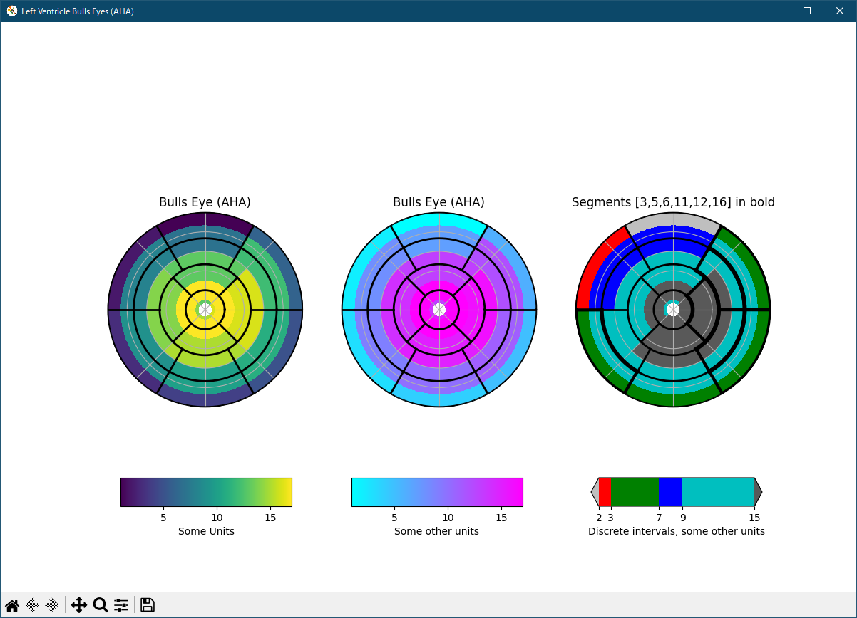
- 参照ページ
pylab_examples_Examples code: leftventricle_bulleye.py
specialty-plots-leftventricle-bullseye-py
- リリースノート
- 2023/11/28 Ver=1.04 Python 3.12.0 (matplotlib 3.8.1)で確認
- 2023/11/28 Ver=1.04 Python 3.11.6 (matplotlib 3.7.1)で確認
- 2023/04/02 Ver=1.03 Python 3.11.2 で確認
- 2020/10/31 Ver=1.01 Python 3.7.8 で確認
- 2018/12/03 Ver=1.01 初版リリース
- 関連ページ