matplotlib Tutorial Tight Layout guide

Information

matplotlib チュートリアル

Our Host


matplotlib Tight Layout guide.	H.Kamifuji .

Tight Layout guide

　タイトレイアウトを使用して、図内にプロットをきれいにフィットさせる方法。

　tight_layout は、サブプロットが図領域に収まるようにサブプロットパラメータを自動的に調整します。これは実験的な機能であり、場合によっては機能しない可能性があります。ティックラベル、軸ラベル、およびタイトルのエクステントのみをチェックします。

　tight_layout の代わりに constrained_layout があります。

目　次

Tight Layout guide

Simple Example

Caveats

Use with GridSpec

Legends and Annotations

Use with AxesGrid1

Colorbar

参照ページ

リリースノート

関連ページ

Simple Example

　matplotlib では、軸の位置（サブプロットを含む）は正規化された Figure 座標で指定されます。あなたの軸のラベルやタイトル（時にはティンカー）は、図の範囲外に出てきて、クリップされることがあります。

import matplotlib.pyplot as plt
import numpy as np

plt.rcParams['savefig.facecolor'] = "0.8"

def example_plot(ax, fontsize=12):
    ax.plot([1, 2])

    ax.locator_params(nbins=3)
    ax.set_xlabel('x-label', fontsize=fontsize)
    ax.set_ylabel('y-label', fontsize=fontsize)
    ax.set_title('Title', fontsize=fontsize)

plt.close('all')
fig, ax = plt.subplots()
example_plot(ax, fontsize=24)

plt.show()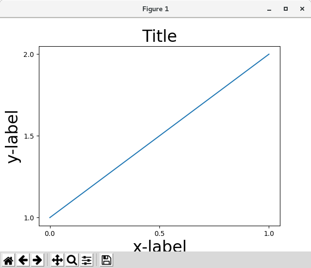

　

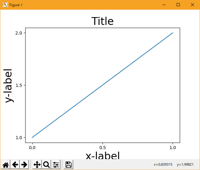
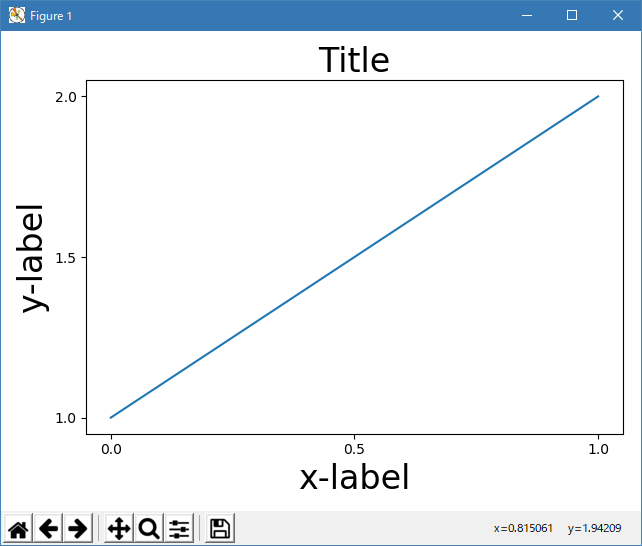
　これを防ぐには、軸の位置を調整する必要があります。サブプロットの場合、これはサブプロットのパラメータを調整することによって行うことができます（軸のエッジを動かして目盛りラベルのためのスペースを確保します）。 Matplotlib v1.1 は自動的にこれを行う新しいコマンド tight_layout() を導入しました。

import matplotlib.pyplot as plt
import numpy as np

plt.rcParams['savefig.facecolor'] = "0.8"

def example_plot(ax, fontsize=12):
    ax.plot([1, 2])

    ax.locator_params(nbins=3)
    ax.set_xlabel('x-label', fontsize=fontsize)
    ax.set_ylabel('y-label', fontsize=fontsize)
    ax.set_title('Title', fontsize=fontsize)

plt.close('all')
fig, ax = plt.subplots()
example_plot(ax, fontsize=24)
plt.tight_layout()

plt.show()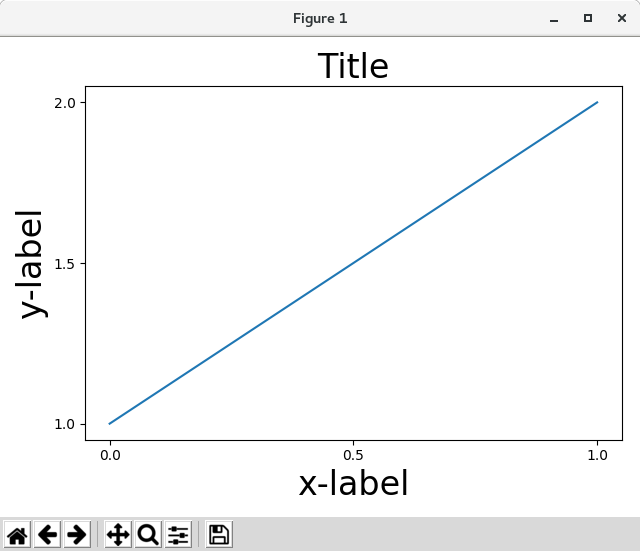

　

　matplotlib.pyplot.tight_layout() は、サブプロットが呼び出されたときにのみそれを調整することに注意してください。 figure を再描画するたびにこの調整を実行するには、fig.set_tight_layout（True）を呼び出すか、figure.autolayout rcParamをTrue に設定します。

　複数のサブプロットがある場合、異なる軸のラベルが重なって表示されることがよくあります。

import matplotlib.pyplot as plt
import numpy as np

plt.rcParams['savefig.facecolor'] = "0.8"

def example_plot(ax, fontsize=12):
    ax.plot([1, 2])

    ax.locator_params(nbins=3)
    ax.set_xlabel('x-label', fontsize=fontsize)
    ax.set_ylabel('y-label', fontsize=fontsize)
    ax.set_title('Title', fontsize=fontsize)

plt.close('all')
fig, ((ax1, ax2), (ax3, ax4)) = plt.subplots(nrows=2, ncols=2)
example_plot(ax1)
example_plot(ax2)
example_plot(ax3)
example_plot(ax4)

plt.show()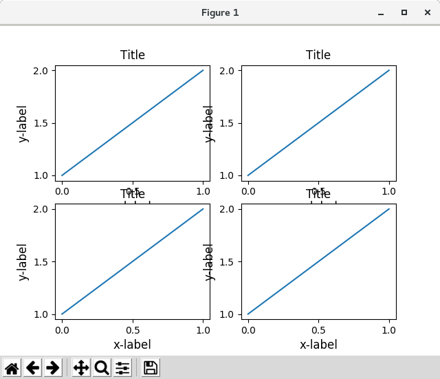

　

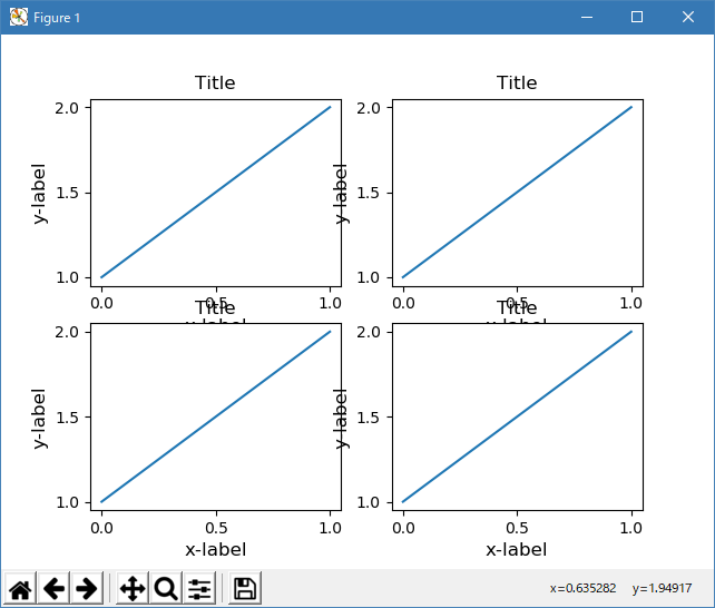
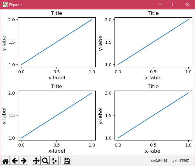
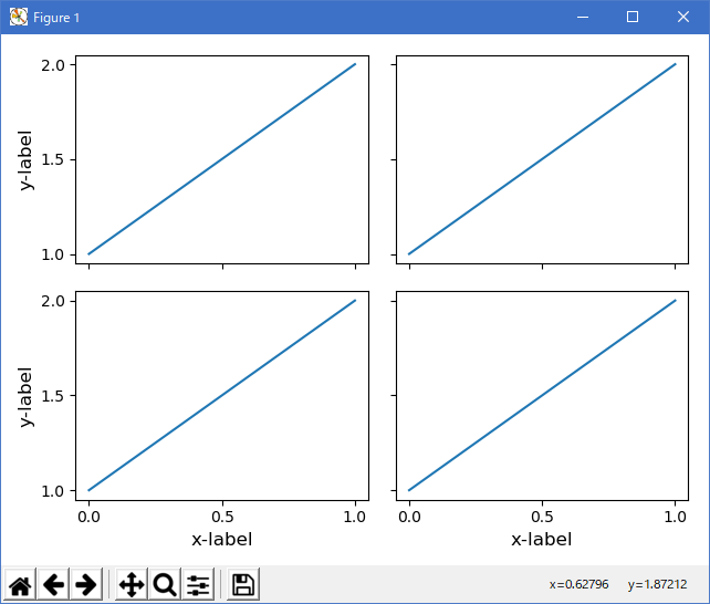
　tight_layout() は、オーバーラップを最小限に抑えるためにサブプロット間の間隔も調整します。

import matplotlib.pyplot as plt
import numpy as np

plt.rcParams['savefig.facecolor'] = "0.8"

def example_plot(ax, fontsize=12):
    ax.plot([1, 2])

    ax.locator_params(nbins=3)
    ax.set_xlabel('x-label', fontsize=fontsize)
    ax.set_ylabel('y-label', fontsize=fontsize)
    ax.set_title('Title', fontsize=fontsize)

plt.close('all')
fig, ((ax1, ax2), (ax3, ax4)) = plt.subplots(nrows=2, ncols=2)
example_plot(ax1)
example_plot(ax2)
example_plot(ax3)
example_plot(ax4)
plt.tight_layout()

plt.show()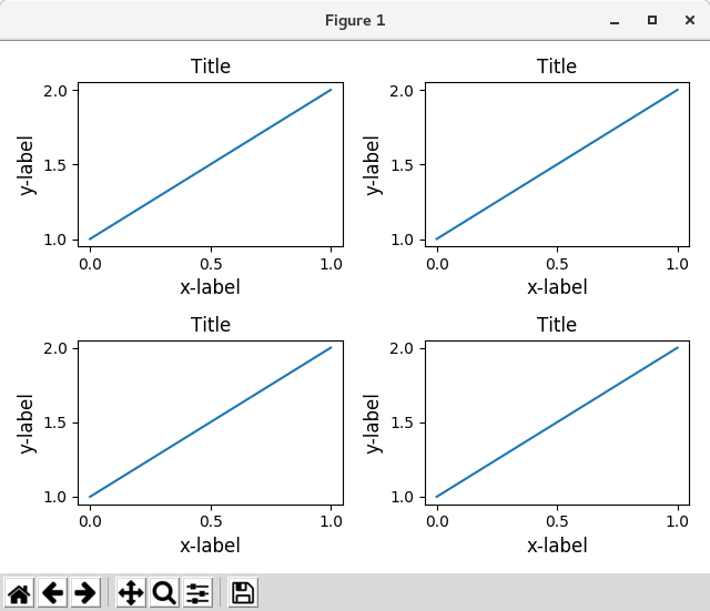

　

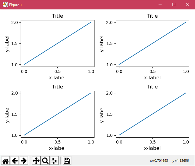
　tight_layout() は、pad、w_pad、h_pad のキーワード引数を取ることができます。これらは、図の境界線の周りとサブプロット間の余分なパディングを制御します。パッドは fontsize の分数で指定します。

import matplotlib.pyplot as plt
import numpy as np

plt.rcParams['savefig.facecolor'] = "0.8"

def example_plot(ax, fontsize=12):
    ax.plot([1, 2])

    ax.locator_params(nbins=3)
    ax.set_xlabel('x-label', fontsize=fontsize)
    ax.set_ylabel('y-label', fontsize=fontsize)
    ax.set_title('Title', fontsize=fontsize)

plt.close('all')
fig, ((ax1, ax2), (ax3, ax4)) = plt.subplots(nrows=2, ncols=2)
example_plot(ax1)
example_plot(ax2)
example_plot(ax3)
example_plot(ax4)
plt.tight_layout(pad=0.4, w_pad=0.5, h_pad=1.0)

plt.show()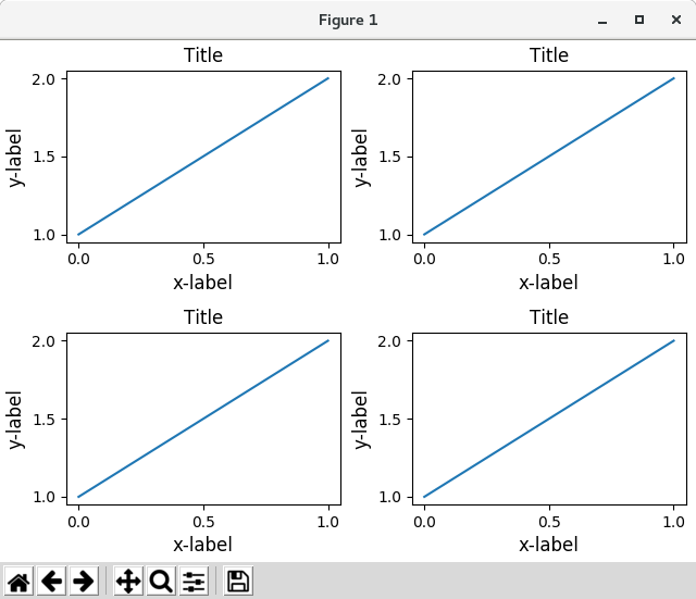

　

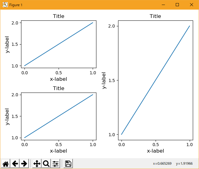
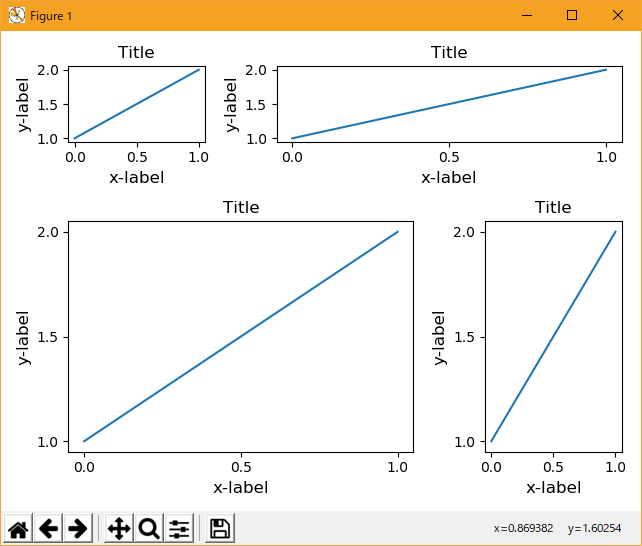
　tight_layout() は、グリッド指定が互換性がある限り、サブプロットのサイズが異なっていても機能します。以下の例では、ax1 とax2 は 2x2 グリッドのサブプロットですが、ax3は1x2 グリッドのサブプロットです。

import matplotlib.pyplot as plt
import numpy as np

plt.rcParams['savefig.facecolor'] = "0.8"

def example_plot(ax, fontsize=12):
    ax.plot([1, 2])

    ax.locator_params(nbins=3)
    ax.set_xlabel('x-label', fontsize=fontsize)
    ax.set_ylabel('y-label', fontsize=fontsize)
    ax.set_title('Title', fontsize=fontsize)

plt.close('all')
fig = plt.figure()

ax1 = plt.subplot(221)
ax2 = plt.subplot(223)
ax3 = plt.subplot(122)

example_plot(ax1)
example_plot(ax2)
example_plot(ax3)

plt.tight_layout()

plt.show()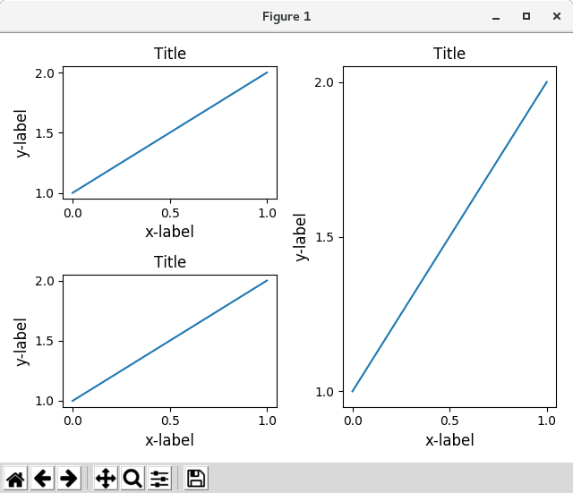

　

　これは subplot2grid() で作成されたサブプロットで動作します。一般に、gridspec（グリッドスペックとその他の関数を使用した図のレイアウトのカスタマイズ）から作成されたサブプロットは機能します。

import matplotlib.pyplot as plt
import numpy as np

plt.rcParams['savefig.facecolor'] = "0.8"

def example_plot(ax, fontsize=12):
    ax.plot([1, 2])

    ax.locator_params(nbins=3)
    ax.set_xlabel('x-label', fontsize=fontsize)
    ax.set_ylabel('y-label', fontsize=fontsize)
    ax.set_title('Title', fontsize=fontsize)

plt.close('all')
fig = plt.figure()

ax1 = plt.subplot2grid((3, 3), (0, 0))
ax2 = plt.subplot2grid((3, 3), (0, 1), colspan=2)
ax3 = plt.subplot2grid((3, 3), (1, 0), colspan=2, rowspan=2)
ax4 = plt.subplot2grid((3, 3), (1, 2), rowspan=2)

example_plot(ax1)
example_plot(ax2)
example_plot(ax3)
example_plot(ax4)

plt.tight_layout()

plt.show()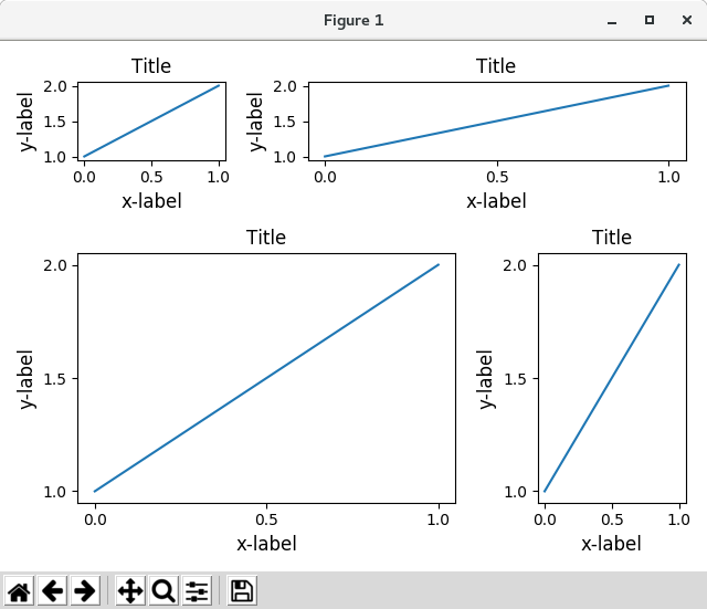

　

　徹底的にテストされているわけではありませんが、aspect！= "auto"（画像付きの軸など）のサブプロットでは機能しているようです。

import matplotlib.pyplot as plt
import numpy as np

plt.rcParams['savefig.facecolor'] = "0.8"

arr = np.arange(100).reshape((10, 10))

plt.close('all')
fig = plt.figure(figsize=(5, 4))

ax = plt.subplot(111)
im = ax.imshow(arr, interpolation="none")

plt.tight_layout()

plt.show()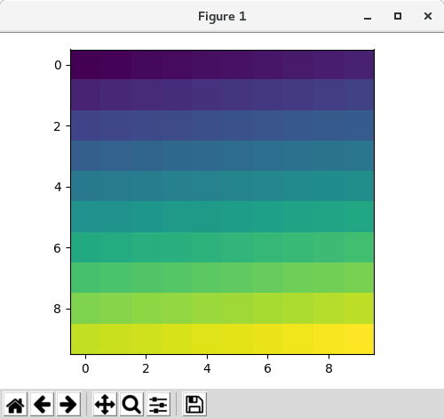

Top

Caveats

tight_layout() は、ティックラベル、軸ラベル、およびタイトルのみを考慮します。従って、他のアーティストはクリップされてもよく、重複してもよい。

ティックラベル、軸ラベル、およびタイトルに必要な余分なスペースが、元の軸の位置とは無関係であると想定しています。これはしばしば真実ですが、そうでない場合はまれです。

pad = 0 はテキストの一部を数ピクセルだけクリップします。これは現在のアルゴリズムのバグまたは制限であり、なぜそれが起こるのかは不明です。一方、少なくとも 0.3 以上のパッドの使用を推奨します。

Top

Use with GridSpec

　GridSpec には独自の tight_layout() メソッドがあります（ pyplot API の tight_layout() も機能します）。

import matplotlib.pyplot as plt
import numpy as np
import matplotlib.gridspec as gridspec


plt.rcParams['savefig.facecolor'] = "0.8"

def example_plot(ax, fontsize=12):
    ax.plot([1, 2])

    ax.locator_params(nbins=3)
    ax.set_xlabel('x-label', fontsize=fontsize)
    ax.set_ylabel('y-label', fontsize=fontsize)
    ax.set_title('Title', fontsize=fontsize)

plt.close('all')
fig = plt.figure()

gs1 = gridspec.GridSpec(2, 1)
ax1 = fig.add_subplot(gs1[0])
ax2 = fig.add_subplot(gs1[1])

example_plot(ax1)
example_plot(ax2)

gs1.tight_layout(fig)

plt.show()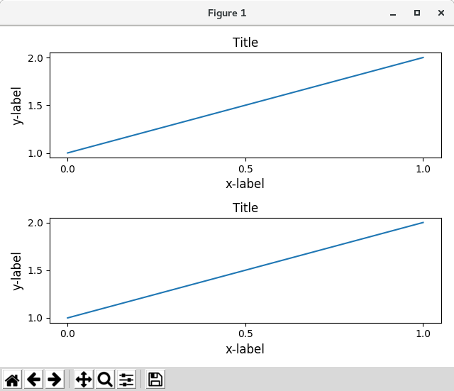

　

　オプションの rect パラメータを指定すると、サブプロットが内部に収まる境界ボックスを指定できます。座標は正規化された Figure 座標でなければならず、デフォルトは（0、0、1、1）です。

import matplotlib.pyplot as plt
import numpy as np
import matplotlib.gridspec as gridspec

plt.rcParams['savefig.facecolor'] = "0.8"

def example_plot(ax, fontsize=12):
    ax.plot([1, 2])

    ax.locator_params(nbins=3)
    ax.set_xlabel('x-label', fontsize=fontsize)
    ax.set_ylabel('y-label', fontsize=fontsize)
    ax.set_title('Title', fontsize=fontsize)

plt.close('all')
fig = plt.figure()

gs1 = gridspec.GridSpec(2, 1)
ax1 = fig.add_subplot(gs1[0])
ax2 = fig.add_subplot(gs1[1])

example_plot(ax1)
example_plot(ax2)

gs1.tight_layout(fig, rect=[0, 0, 0.5, 1])

plt.show()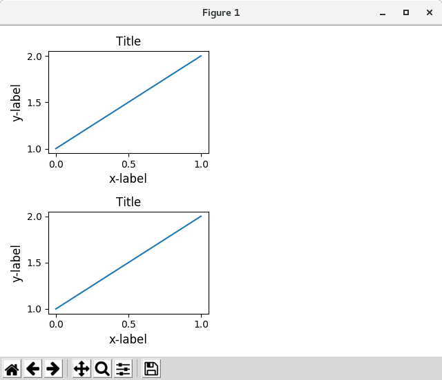

　

　たとえば、これは複数のグリッド・スペックを持つFigureに使用できます。

import matplotlib.pyplot as plt
import numpy as np
import matplotlib.gridspec as gridspec

plt.rcParams['savefig.facecolor'] = "0.8"

def example_plot(ax, fontsize=12):
    ax.plot([1, 2])

    ax.locator_params(nbins=3)
    ax.set_xlabel('x-label', fontsize=fontsize)
    ax.set_ylabel('y-label', fontsize=fontsize)
    ax.set_title('Title', fontsize=fontsize)

plt.close('all')
fig = plt.figure()

gs1 = gridspec.GridSpec(2, 1)
ax1 = fig.add_subplot(gs1[0])
ax2 = fig.add_subplot(gs1[1])

example_plot(ax1)
example_plot(ax2)

gs1.tight_layout(fig, rect=[0, 0, 0.5, 1])

gs2 = gridspec.GridSpec(3, 1)

for ss in gs2:
    ax = fig.add_subplot(ss)
    example_plot(ax)
    ax.set_title("")
    ax.set_xlabel("")

ax.set_xlabel("x-label", fontsize=12)

gs2.tight_layout(fig, rect=[0.5, 0, 1, 1], h_pad=0.5)

# We may try to match the top and bottom of two grids ::
top = min(gs1.top, gs2.top)
bottom = max(gs1.bottom, gs2.bottom)

gs1.update(top=top, bottom=bottom)
gs2.update(top=top, bottom=bottom)

plt.show()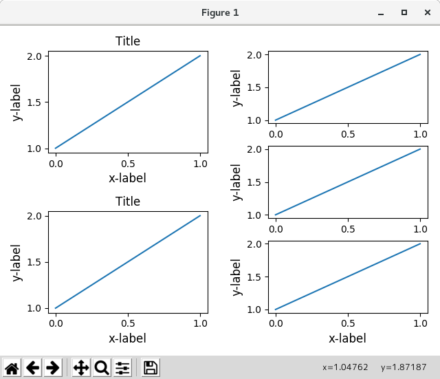

　

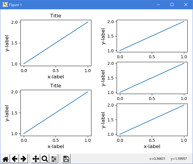
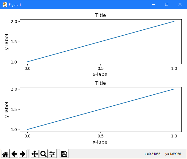
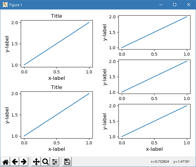
　これは主に十分なはずですが、上下を調整するには hspace も調整する必要があります。 hspace＆vspace を更新するには、updated rect 引数で tight_layout() を再度呼び出します。 rect 引数では、ティックラベルなどの領域を指定していることに注意してください。したがって、上からのボトムと各グリッドの下端との差でボトム（通常の場合は0）を増やします。トップにも同じこと。

import matplotlib.pyplot as plt
import numpy as np
import matplotlib.gridspec as gridspec

plt.rcParams['savefig.facecolor'] = "0.8"

def example_plot(ax, fontsize=12):
    ax.plot([1, 2])

    ax.locator_params(nbins=3)
    ax.set_xlabel('x-label', fontsize=fontsize)
    ax.set_ylabel('y-label', fontsize=fontsize)
    ax.set_title('Title', fontsize=fontsize)

plt.close('all')
fig = plt.gcf()

gs1 = gridspec.GridSpec(2, 1)
ax1 = fig.add_subplot(gs1[0])
ax2 = fig.add_subplot(gs1[1])

example_plot(ax1)
example_plot(ax2)

gs1.tight_layout(fig, rect=[0, 0, 0.5, 1])

gs2 = gridspec.GridSpec(3, 1)

for ss in gs2:
    ax = fig.add_subplot(ss)
    example_plot(ax)
    ax.set_title("")
    ax.set_xlabel("")

ax.set_xlabel("x-label", fontsize=12)

gs2.tight_layout(fig, rect=[0.5, 0, 1, 1], h_pad=0.5)

top = min(gs1.top, gs2.top)
bottom = max(gs1.bottom, gs2.bottom)

gs1.update(top=top, bottom=bottom)
gs2.update(top=top, bottom=bottom)

top = min(gs1.top, gs2.top)
bottom = max(gs1.bottom, gs2.bottom)

gs1.tight_layout(fig, rect=[None, 0 + (bottom-gs1.bottom),
                            0.5, 1 - (gs1.top-top)])
gs2.tight_layout(fig, rect=[0.5, 0 + (bottom-gs2.bottom),
                            None, 1 - (gs2.top-top)],
                 h_pad=0.5)

plt.show()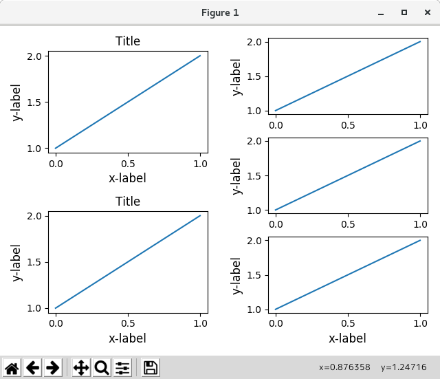

Top

Legends and Annotations

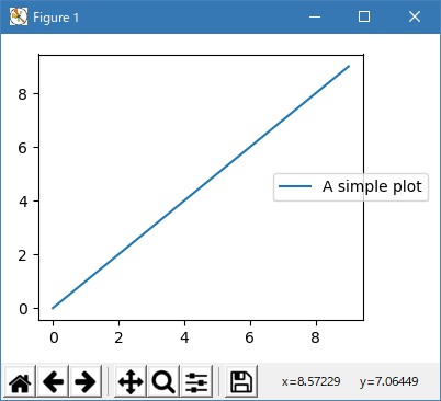
　Pre Matplotlih 2.2 では、レイアウトを決めるバウンディングボックス計算から凡例と注釈が除外されました。その後、これらのアーティストは計算に追加されましたが、時にはそれらを含めることは望ましくありません。たとえば、この場合、凡例のためのスペースを確保するために、軸を少しだけ砕くのが良いかもしれません：

import matplotlib.pyplot as plt
import numpy as np
import matplotlib.gridspec as gridspec

plt.rcParams['savefig.facecolor'] = "0.8"

def example_plot(ax, fontsize=12):
    ax.plot([1, 2])

    ax.locator_params(nbins=3)
    ax.set_xlabel('x-label', fontsize=fontsize)
    ax.set_ylabel('y-label', fontsize=fontsize)
    ax.set_title('Title', fontsize=fontsize)

plt.close('all')
fig, ax = plt.subplots(figsize=(4, 3))
lines = ax.plot(range(10), label='A simple plot')
ax.legend(bbox_to_anchor=(0.7, 0.5), loc='center left',)
fig.tight_layout()

plt.show()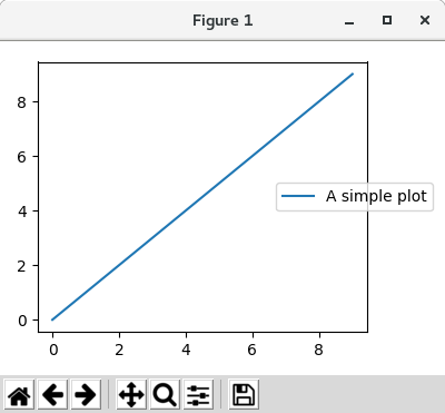

　

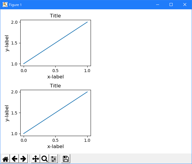
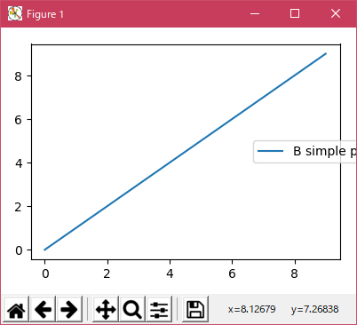
　しかし、時にはこれは望ましくないことがあります（fig.savefig（ 'outname.png'、bbox_inches = 'tight' ）を使用する場合）。凡例をバウンディングボックス計算から削除するには、その境界 leg.set_in_layout（False）を設定するだけで、凡例は無視されます。

import matplotlib.pyplot as plt
import numpy as np
import matplotlib.gridspec as gridspec

plt.rcParams['savefig.facecolor'] = "0.8"

def example_plot(ax, fontsize=12):
    ax.plot([1, 2])

    ax.locator_params(nbins=3)
    ax.set_xlabel('x-label', fontsize=fontsize)
    ax.set_ylabel('y-label', fontsize=fontsize)
    ax.set_title('Title', fontsize=fontsize)

plt.close('all')
fig, ax = plt.subplots(figsize=(4, 3))
lines = ax.plot(range(10), label='B simple plot')
leg = ax.legend(bbox_to_anchor=(0.7, 0.5), loc='center left',)
leg.set_in_layout(False)
fig.tight_layout()

plt.show()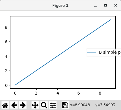

Top

Use with AxesGrid1

　限られているものの、axes_grid1 ツールキットもサポートされています。

import matplotlib.pyplot as plt
import numpy as np
import matplotlib.gridspec as gridspec
from mpl_toolkits.axes_grid1 import Grid

plt.rcParams['savefig.facecolor'] = "0.8"

def example_plot(ax, fontsize=12):
    ax.plot([1, 2])

    ax.locator_params(nbins=3)
    ax.set_xlabel('x-label', fontsize=fontsize)
    ax.set_ylabel('y-label', fontsize=fontsize)
    ax.set_title('Title', fontsize=fontsize)

plt.close('all')
fig = plt.figure()
grid = Grid(fig, rect=111, nrows_ncols=(2, 2),
            axes_pad=0.25, label_mode='L',
            )

for ax in grid:
    example_plot(ax)
    ax.title.set_visible(False)

plt.tight_layout()

plt.show()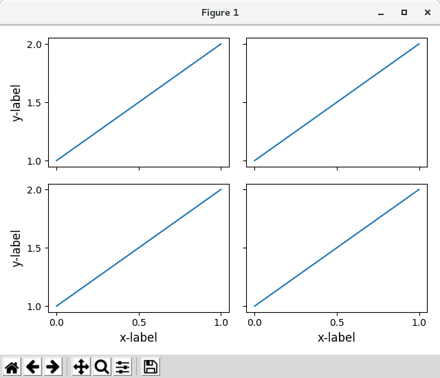

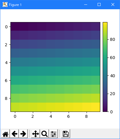
Top

Colorbar

　colorbar() コマンドでカラーバーを作成すると、作成されたカラーバーはサブプロットではなく Axes のインスタンスなので、tight_layout は機能しません。 Matplotlib v1.1では、gridspec を使用してサブプロットとしてカラーバーを作成することができます。

import matplotlib.pyplot as plt
import numpy as np

plt.rcParams['savefig.facecolor'] = "0.8"

arr = np.arange(100).reshape((10, 10))

plt.close('all')
fig = plt.figure(figsize=(4, 4))
im = plt.imshow(arr, interpolation="none")

plt.colorbar(im, use_gridspec=True)

plt.tight_layout()

plt.show()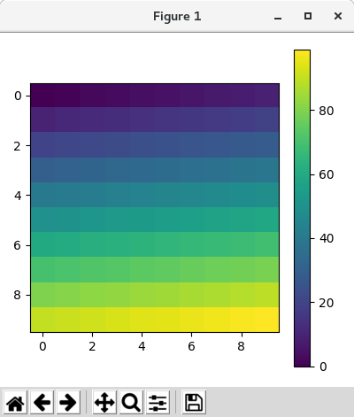

　

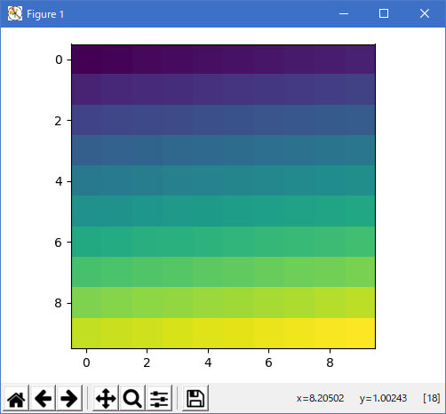
　AxesGrid1 ツールキットを使用して、カラーバーの軸を明示的に作成することもできます。

import matplotlib.pyplot as plt
import numpy as np
from mpl_toolkits.axes_grid1 import make_axes_locatable

plt.rcParams['savefig.facecolor'] = "0.8"

arr = np.arange(100).reshape((10, 10))

plt.close('all')
fig = plt.figure(figsize=(4, 4))
im = plt.imshow(arr, interpolation="none")

divider = make_axes_locatable(plt.gca())
cax = divider.append_axes("right", "5%", pad="3%")
plt.colorbar(im, cax=cax)

plt.tight_layout()

plt.show()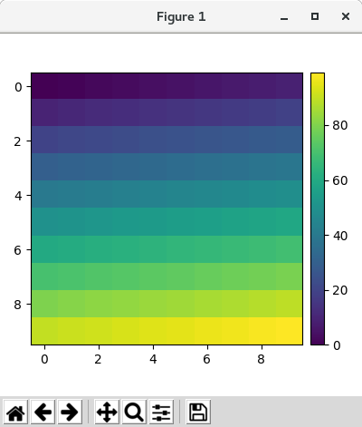

　

　スクリプトの合計実行時間：（0分1.019秒）

Top

参照ページ

Tight Layout guide

リリースノート
2023/03/11 Ver=1.03 Python 3.11.2 で確認

2020/10/28 Ver=1.01 Python 3.7.8 で確認

2018/11/08 Ver=1.01 初版リリース

関連ページ
Python インストール Windows 版

Python インストール Linux 版

MAX_PATH を除去する

Top