|
|
matplotlib Customizing Figure Layouts Using GridSpec and Other Functions. |
H.Kamifuji . |
- 目 次
- Customizing Figure Layouts Using GridSpec and Other Functions
グリッド型の軸の組み合わせを作成する方法。
- subplots()
- おそらく主な機能は、図や軸を作成するために使用されます。 これは matplotlib.pyplot.subplot() と似ていますが、Figure 上のすべての軸を作成して一度に配置します。 matplotlib.Figure.subplots も参照してください。
- GridSpec
- サブプロットが配置されるグリッドのジオメトリを指定します。 グリッドの行数と列数を設定する必要があります。 任意選択で、サブプロットレイアウトパラメータ(例えば、左、右など)を調整することができる。
- SubplotSpec
- 指定された GridSpec 内のサブプロットの位置を指定します。
- subplot2grid()
- subplot() と似ていますが、0 ベースのインデックスを使用し、サブプロットを複数のセルを占めるようにするヘルパー関数です。 この関数はこのチュートリアルでは扱いません。
import matplotlib
import matplotlib.pyplot as plt
import matplotlib.gridspec as gridspec
- Basic Quickstart Guide
これらの最初の 2 つの例は、subplots() と gridspec の両方を使用して基本2行2列グリッドを作成する方法を示しています。
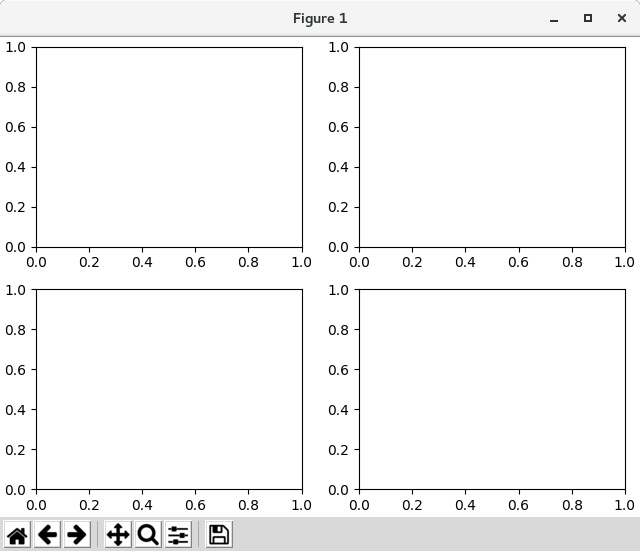
subplots() を使用することは非常に簡単です。 これは、Figure インスタンスと Axes オブジェクトの配列を返します。
import matplotlib
import matplotlib.pyplot as plt
import matplotlib.gridspec as gridspec

fig1, f1_axes = plt.subplots(ncols=2, nrows=2, constrained_layout=True)

plt.show()
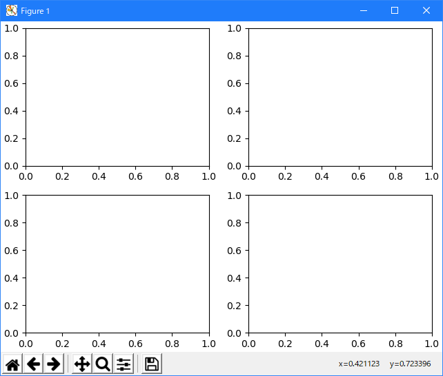
このような単純なユースケースの場合、gridspec はおそらく過度に冗長です。 Figure と GridSpec インスタンスを別々に作成し、次に gridspec インスタンスの要素を add_subplot() メソッドに渡して Axes オブジェクトを作成する必要があります。 gridspec の要素は、numpy 配列とほぼ同じ方法でアクセスされます。
import matplotlib
import matplotlib.pyplot as plt
import matplotlib.gridspec as gridspec

fig2 = plt.figure(constrained_layout=True)
spec2 = gridspec.GridSpec(ncols=2, nrows=2, figure=fig2)
f2_ax1 = fig2.add_subplot(spec2[0, 0])
f2_ax2 = fig2.add_subplot(spec2[0, 1])
f2_ax3 = fig2.add_subplot(spec2[1, 0])
f2_ax4 = fig2.add_subplot(spec2[1, 1])

plt.show()


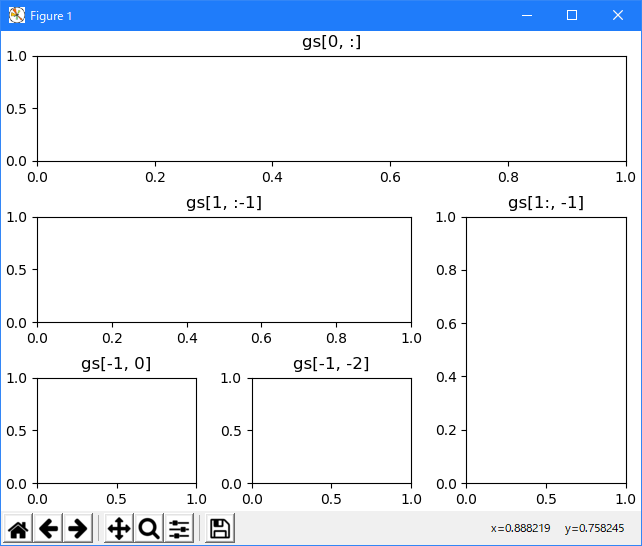
gridspec の機能は、行と列にまたがるサブプロットを作成することができます。 各サブプロットが占有するグリッドスペックの一部を選択するための Numpy slice シンタックスに注意してください。
gridspec.GridSpec の代わりに便利なメソッド Figure.add_gridspec を使用して、潜在的にユーザにインポートを保存し、名前空間をよりきれいに保つことに注意してください。
import matplotlib
import matplotlib.pyplot as plt
import matplotlib.gridspec as gridspec

fig3 = plt.figure(constrained_layout=True)
gs = fig3.add_gridspec(3, 3)
f3_ax1 = fig3.add_subplot(gs[0, :])
f3_ax1.set_title('gs[0, :]')
f3_ax2 = fig3.add_subplot(gs[1, :-1])
f3_ax2.set_title('gs[1, :-1]')
f3_ax3 = fig3.add_subplot(gs[1:, -1])
f3_ax3.set_title('gs[1:, -1]')
f3_ax4 = fig3.add_subplot(gs[-1, 0])
f3_ax4.set_title('gs[-1, 0]')
f3_ax5 = fig3.add_subplot(gs[-1, -2])
f3_ax5.set_title('gs[-1, -2]')

plt.show()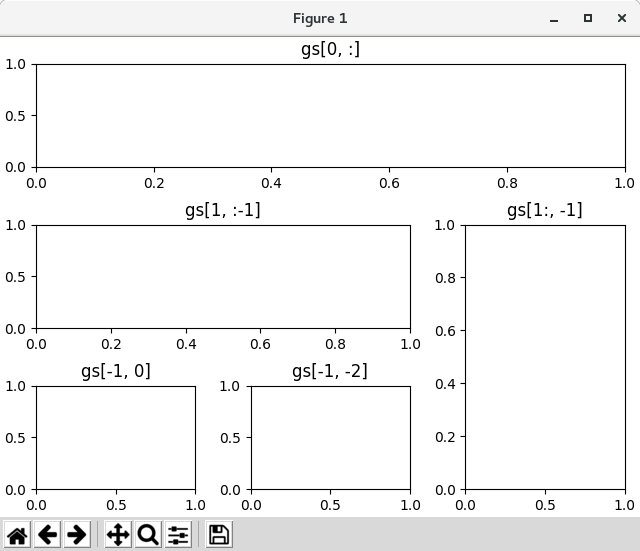
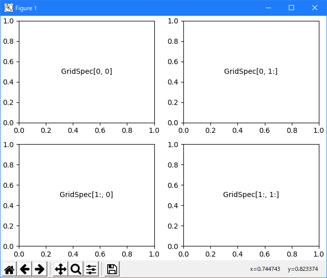
gridspec は、いくつかの方法で異なる幅のサブプロットを作成するためにも不可欠です。
ここに示す方法は、上記の方法と似ていて、均一なグリッド指定を初期化し、numpy インデックスとスライスを使用して、指定されたサブプロットに対して複数の "セル"を割り当てます。
import matplotlib
import matplotlib.pyplot as plt
import matplotlib.gridspec as gridspec

fig4 = plt.figure(constrained_layout=True)
spec4 = fig4.add_gridspec(ncols=2, nrows=2)
anno_opts = dict(xy=(0.5, 0.5), xycoords='axes fraction',
                 va='center', ha='center')

f4_ax1 = fig4.add_subplot(spec4[0, 0])
f4_ax1.annotate('GridSpec[0, 0]', **anno_opts)
fig4.add_subplot(spec4[0, 1]).annotate('GridSpec[0, 1:]', **anno_opts)
fig4.add_subplot(spec4[1, 0]).annotate('GridSpec[1:, 0]', **anno_opts)
fig4.add_subplot(spec4[1, 1]).annotate('GridSpec[1:, 1:]', **anno_opts)

plt.show()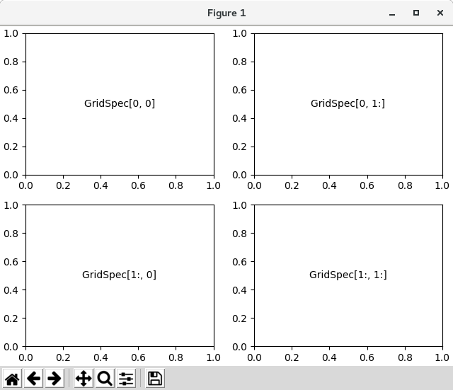
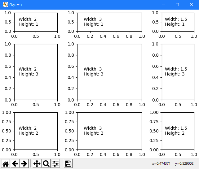
別のオプションは、width_ratiosとheight_ratios パラメータを使用することです。 これらのキーワード引数は数字のリストです。 絶対値は無意味であり、相対的な比率だけが重要であることに注意してください。 つまり、width_ratios=[2,4,8] は、幅の広い図では width_ratios=[1,2,4] と等価です。 デモンストレーションのために、後で必要としないので、for ループ内で盲目的に軸を作成します。
import matplotlib
import matplotlib.pyplot as plt
import matplotlib.gridspec as gridspec

fig5 = plt.figure(constrained_layout=True)
widths = [2, 3, 1.5]
heights = [1, 3, 2]
spec5 = fig5.add_gridspec(ncols=3, nrows=3, width_ratios=widths,
                          height_ratios=heights)
for row in range(3):
    for col in range(3):
        ax = fig5.add_subplot(spec5[row, col])
        label = 'Width: {}\nHeight: {}'.format(widths[col], heights[row])
        ax.annotate(label, (0.1, 0.5), xycoords='axes fraction', va='center')

plt.show()
width_ratios と height_ratios を使用することを学ぶことは、トップレベルの関数 subplots() がgridspec_kw パラメータ内でそれらを受け入れるので、特に便利です。 そのため、GridSpec で受け入れられたパラメータは、gridspec_kw パラメータを介して subplots() に渡すことができます。 この例では、gridspec インスタンスを直接使用せずに前のFigureを再作成します。
import matplotlib
import matplotlib.pyplot as plt
import matplotlib.gridspec as gridspec

widths = [2, 3, 1.5]
heights = [1, 3, 2]

gs_kw = dict(width_ratios=widths, height_ratios=heights)
fig6, f6_axes = plt.subplots(ncols=3, nrows=3, constrained_layout=True,
        gridspec_kw=gs_kw)
for r, row in enumerate(f6_axes):
    for c, ax in enumerate(row):
        label = 'Width: {}\nHeight: {}'.format(widths[c], heights[r])
        ax.annotate(label, (0.1, 0.5), xycoords='axes fraction', va='center')

plt.show()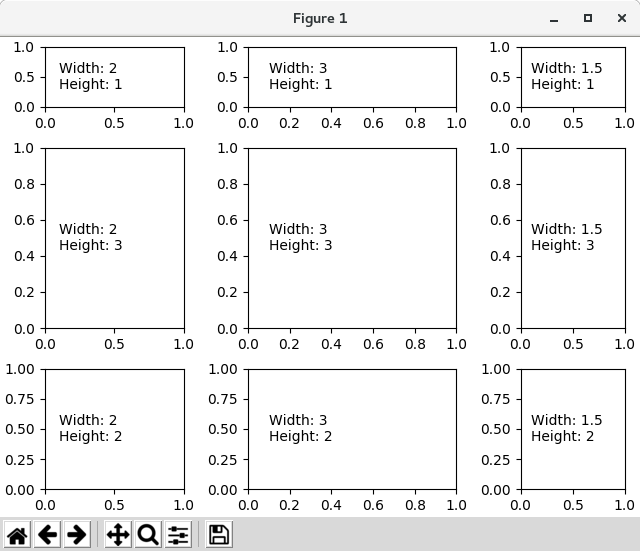

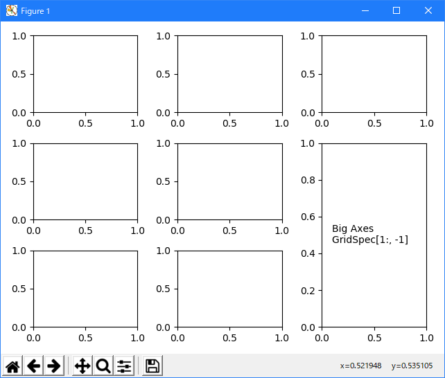
サブプロットを使用してサブプロットの大部分を作成し、いくつかを削除して結合する方が便利な場合があるので、サブプロットと gridspec の方法を組み合わせることができます。 ここでは、最後の列の下の2つの軸を組み合わせたレイアウトを作成します。
import matplotlib
import matplotlib.pyplot as plt
import matplotlib.gridspec as gridspec

fig7, f7_axs = plt.subplots(ncols=3, nrows=3)
gs = f7_axs[1, 2].get_gridspec()
# remove the underlying axes
for ax in f7_axs[1:, -1]:
    ax.remove()
axbig = fig7.add_subplot(gs[1:, -1])
axbig.annotate('Big Axes \nGridSpec[1:, -1]', (0.1, 0.5),
               xycoords='axes fraction', va='center')

fig7.tight_layout()

plt.show()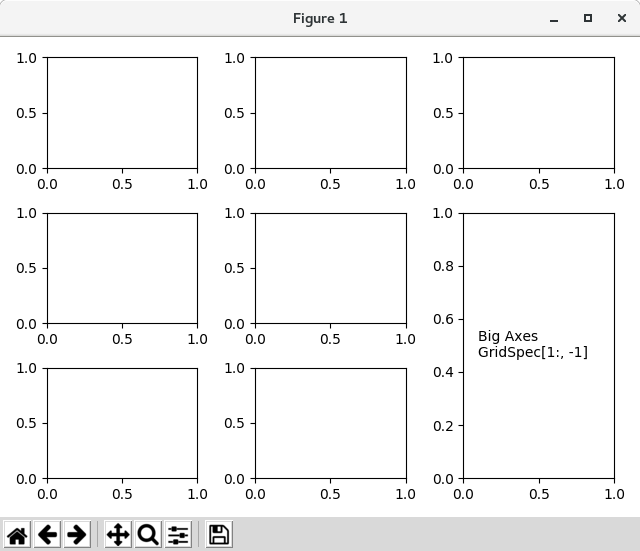
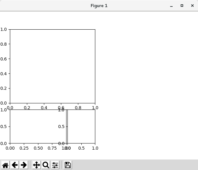
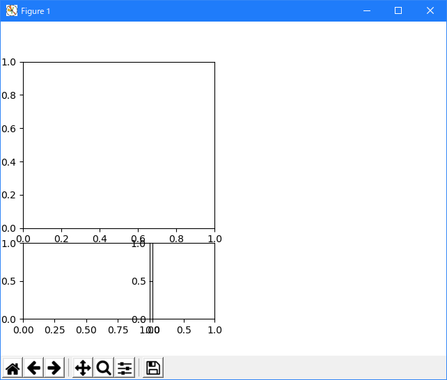
- Fine Adjustments to a Gridspec Layout
GridSpec を明示的に使用する場合は、GridSpec から作成されたサブプロットのレイアウトパラメータを調整できます。 このオプションは constrained_layout または Figure.tight_layout と互換性がないことに注意してください。どちらも図を埋めるためにサブプロットサイズを調整します。
import matplotlib
import matplotlib.pyplot as plt
import matplotlib.gridspec as gridspec

fig8 = plt.figure(constrained_layout=False)
gs1 = fig8.add_gridspec(nrows=3, ncols=3, left=0.05, right=0.48, wspace=0.05)
f8_ax1 = fig8.add_subplot(gs1[:-1, :])
f8_ax2 = fig8.add_subplot(gs1[-1, :-1])
f8_ax3 = fig8.add_subplot(gs1[-1, -1])

plt.show()
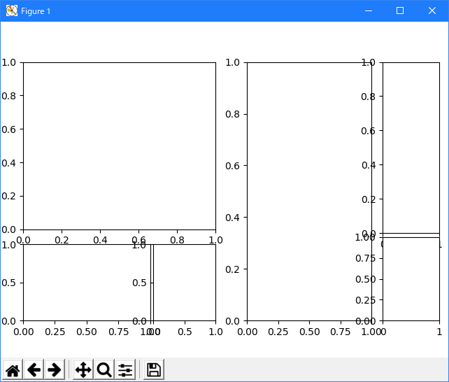
これは subplots_adjust() と似ていますが、指定された GridSpec から作成されたサブプロットにのみ影響します。
たとえば、この図の左辺と右辺を比較します。
import matplotlib
import matplotlib.pyplot as plt
import matplotlib.gridspec as gridspec

fig9 = plt.figure(constrained_layout=False)
gs1 = fig9.add_gridspec(nrows=3, ncols=3, left=0.05, right=0.48,
                        wspace=0.05)
f9_ax1 = fig9.add_subplot(gs1[:-1, :])
f9_ax2 = fig9.add_subplot(gs1[-1, :-1])
f9_ax3 = fig9.add_subplot(gs1[-1, -1])

gs2 = fig9.add_gridspec(nrows=3, ncols=3, left=0.55, right=0.98,
                        hspace=0.05)
f9_ax4 = fig9.add_subplot(gs2[:, :-1])
f9_ax5 = fig9.add_subplot(gs2[:-1, -1])
f9_ax6 = fig9.add_subplot(gs2[-1, -1])

plt.show()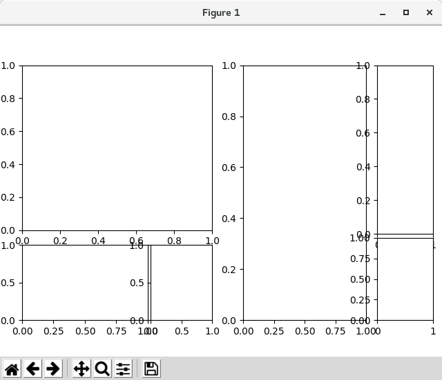
- GridSpec using SubplotSpec
SubplotSpec から GridSpec を作成することができます。その場合、そのレイアウトパラメータは、指定された SubplotSpec の位置のレイアウトパラメータに設定されます。
これは、より冗長な gridspec.GridSpecFromSubplotSpec からも利用できます。
import matplotlib
import matplotlib.pyplot as plt
import matplotlib.gridspec as gridspec

fig10 = plt.figure(constrained_layout=True)
gs0 = fig10.add_gridspec(1, 2)

gs00 = gs0[0].subgridspec(2, 3)
gs01 = gs0[1].subgridspec(3, 2)

for a in range(2):
    for b in range(3):
        fig10.add_subplot(gs00[a, b])
        fig10.add_subplot(gs01[b, a])

plt.show()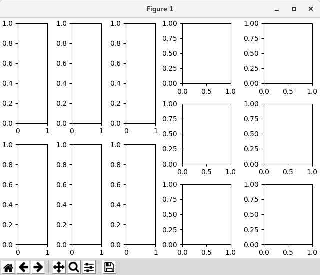
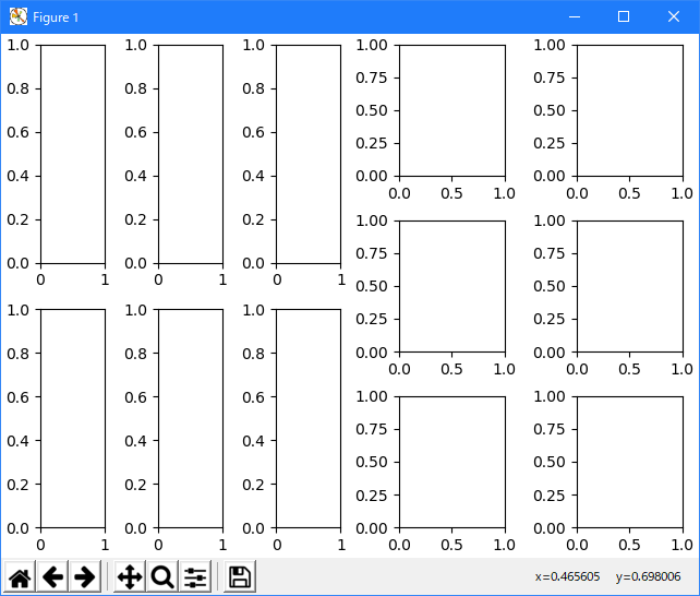
- A Complex Nested GridSpec using SubplotSpec
ここでは、より洗練されたネストされたGridSpecの例を示します。ここでは、内側の3x3グリッドのそれぞれに適切な背を隠すことによって、 外側の4x4グリッドの各セルの周りにボックスを配置します。
import matplotlib
import matplotlib.pyplot as plt
import matplotlib.gridspec as gridspec
import numpy as np
from itertools import product


def squiggle_xy(a, b, c, d, i=np.arange(0.0, 2*np.pi, 0.05)):
    return np.sin(i*a)*np.cos(i*b), np.sin(i*c)*np.cos(i*d)


fig11 = plt.figure(figsize=(8, 8), constrained_layout=False)

# gridspec inside gridspec
outer_grid = fig11.add_gridspec(4, 4, wspace=0.0, hspace=0.0)

for i in range(16):
    inner_grid = outer_grid[i].subgridspec(3, 3, wspace=0.0, hspace=0.0)
    a, b = int(i/4)+1, i % 4+1
    for j, (c, d) in enumerate(product(range(1, 4), repeat=2)):
        ax = plt.Subplot(fig11, inner_grid[j])
        ax.plot(*squiggle_xy(a, b, c, d))
        ax.set_xticks([])
        ax.set_yticks([])
        fig11.add_subplot(ax)

all_axes = fig11.get_axes()

# show only the outside spines
for ax in all_axes:
    for sp in ax.spines.values():
        sp.set_visible(False)
    if ax.is_first_row():
        ax.spines['top'].set_visible(True)
    if ax.is_last_row():
        ax.spines['bottom'].set_visible(True)
    if ax.is_first_col():
        ax.spines['left'].set_visible(True)
    if ax.is_last_col():
        ax.spines['right'].set_visible(True)

plt.show()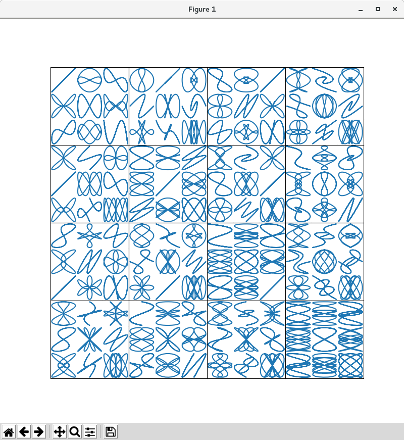
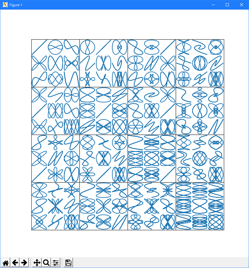
Python 3.11.2 見直しました。上記のコードでは、下記のエラーが発生します。
Traceback (most recent call last):
File "_:\Figure_Layouts_11.py", line 33, in
if ax.is_first_row():
^^^^^^^^^^^^^^^
AttributeError: 'Axes' object has no attribute 'is_first_row'import matplotlib import matplotlib.pyplot as plt import matplotlib.gridspec as gridspec import numpy as np from itertools import product def squiggle_xy(a, b, c, d, i=np.arange(0.0, 2*np.pi, 0.05)): return np.sin(i*a)*np.cos(i*b), np.sin(i*c)*np.cos(i*d) fig = plt.figure(figsize=(8, 8), constrained_layout=False) outer_grid = fig.add_gridspec(4, 4, wspace=0, hspace=0) for a in range(4): for b in range(4): # gridspec inside gridspec inner_grid = outer_grid[a, b].subgridspec(3, 3, wspace=0, hspace=0) axs = inner_grid.subplots() # Create all subplots for the inner grid. for (c, d), ax in np.ndenumerate(axs): ax.plot(*squiggle_xy(a + 1, b + 1, c + 1, d + 1)) ax.set(xticks=[], yticks=[]) # show only the outside spines for ax in fig.get_axes(): ss = ax.get_subplotspec() ax.spines.top.set_visible(ss.is_first_row()) ax.spines.bottom.set_visible(ss.is_last_row()) ax.spines.left.set_visible(ss.is_first_col()) ax.spines.right.set_visible(ss.is_last_col()) plt.show() 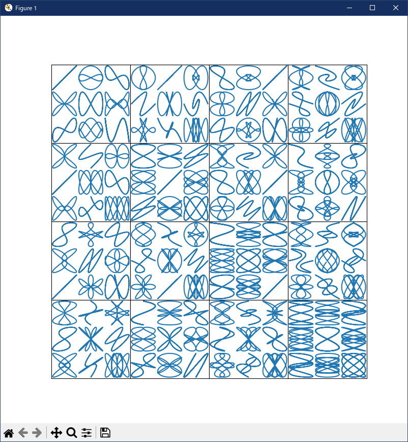
- References
この例では、以下の関数とメソッドの使用法を示しています。
- 参照ページ
Customizing Figure Layouts Using GridSpec and Other Functions
- リリースノート
- 2023/03/22 Ver=1.03 Python 3.11.2 で確認
- 2020/10/28 Ver=1.01 Python 3.7.8 で確認
- 2018/11/08 Ver=1.01 初版リリース
- 関連ページ